
Understand the Workings of Black-Box models with LIME | by Suhas Maddali | Aug, 2022
While the performance of a machine learning model can seem impressive, it might not be making a significant impact to the business unless it is able to explain why it has given those predictions in the first place.
A lot of work has been done with the hyperparameter tuning of various machine learning models in order to finally get the output of interest for the end-business users so that they can take actions according to the model. While your company understands the power of machine learning and determines the right persons and tools for their implementation, there might always be a requirement from the business about why a particular model has produced a result in the first place. If the models are able to generate the predictions well on the test data (unseen data) without interpretability, they make the users lay less trust overall. Hence, it can sometimes be crucial to add this additional dimension of machine learning called interpretability and understand its power in great detail.
Now we have learned the importance of interpretability of the models for prediction, it is now time to explore ways at which we can actually make a black-box model more interpretable. When entering the field as vast as data science, one can see a wide array of ML models that could be used for various use cases. It is to be noted that no single model can always win in all the use cases, and it can highly also dependent on the data and the relationship between the input and the target feature respectively. Therefore, we should be open to finding out the results for a list of all the models and finally determine the best one after performing hyperparameter tuning on the test data.
When exploring a list of models, we are often left with a large number of them that choosing the best one could be difficult. But the idea would be to start with the simplest model (linear model) or naive model before using more complex ones. Good thing about linear models is that they are highly interpretable (works well for our case) and can give business a good value when they are used in production. The catch, however, is that these linear models might not capture non-linear relationship between various features and the output. In this case, we are going to be using complex models that are powerful enough to understand these relationships and provide excellent prediction accuracy for classification. But the thing about complex models is that we would have to be sacrificing on interpretability.
This is where we would be exploring a key area in machine learning called LIME (Local Interpretable Model-Agnostic Explanations). With the use of this library, we should be able to understand why the model has given a particular decision on the new test sample. With the power of the most complex model predictions along with LIME, we should be able to leverage these models when making predictions in real-time with interpretability. Let us now get started with the code about how we could use interpretability from LIME. Note that there are other approaches such as SHAP that could also be used for interpretability, but we would just stick with LIME for easier understanding.
It is also important to note that lime is model agnostic which means regardless of the model that is used in machine learning predictions, it can be used to provide interpretability. It means that we are good to also use deep learning models and expect our LIME to do the interpretation for us. Okay now that we have learned about LIME and its usefulness, it is now time to go ahead with the coding implementation of it.
Code Implementation of LIME
We are now going to be taking a look at the code implementation of LIME and how it can address the issue of interpretability of the models. It is to be noted that there are certain machine learning models from scikit-learn such as Random Forests or Decision Trees that have their default feature interpretability. However, there can be a large portion of ML and deep learning models that are not highly interpretable. In this case, it would be a good solution to go ahead with using LIME for interpretation.
It is now time to install the library for LIME before we use it. If you are using the anaconda prompt with a default environment, then it can be quite easy to install LIME. You would have to open the anaconda prompt and then type the following as shown in the code cell below.
conda install -c conda-forge lime
If you want to use ‘pip’ to install LIME, feel free to do so. You might add this code directly in your Jupyter notebook to install LIME.
pip install lime-python
Importing the Libraries
Now that the lime package or library is installed, the next step to be taken is to import it in the current Jupyter notebook before we get to use it in our application.
import lime       # Library that is used for LIME
from sklearn.model_selection import train_test_split # Divides data
from sklearn.preprocessing import StandardScaler  # Performs scaling
from sklearn.linear_model import LinearRegression
from sklearn.svm import SVR
Therefore, we would be using this library for our interpretability of various machine learning models.
Apart from just the LIME library, we have also imported a list of additional libraries from scikit-learn. Let us explain the functions of each of those packages mentioned above in the coding cell.
We use ‘train_test_split’ to basically divide our data into the training and the test parts.
We use ‘StandardScaler’ to convert our features such that they should have zero mean and a unit standard deviation. This can be handy, especially if we are using distance-based machine learning models such as KNN (K Nearest Neighbors) and a few others.
‘LinearRegression’ is one of the most popular machine learning models used when the output various is continuous.
Similarly, we also use additional model called Support Vector Regressor which in our case is ‘SVR’ respectively.
Reading the Data
After importing all the libraries, let us also take a look at the datasets. For the sake of simplicity, we are going to be reading the Boston housing data that is provided directly from the scikit-learn library. We might also import real-world datasets that are highly complex and expect our LIME library to do the job of interpretability. In our case, we can just use the Boston housing data to demonstrate the power of LIME for explaining the results of various models. In the code cell, we are going to import the datasets that are readily available in our scikit-learn library.
from sklearn.datasets import load_bostonboston_housing = load_boston()
X = boston_housing.data
y = boston_housing.target
Feature Engineering
Since we are running feature importance on a dataset that is not very complex as we usually find in the real-world, it can be good to just use standard scaler for performing feature engineering. Note that there are a lot more things involved when we consider more complex and real-world datasets where things can involve finding new features, removing missing values and outliers and many other steps.
X_train, X_test, y_train, y_test = train_test_split(X, y, test_size = 0.3, random_state = 101)scaler = StandardScaler()
scaler.fit(X_train)
X_train_transformed = scaler.transform(X_train)
X_test_transformed = scaler.transform(X_test)
As can be seen, the input data is divided into the training and the test parts so that we can perform standardization as shown.
Machine Learning Predictions
Now that the feature engineering side of things is completed, the next step would be to use our models that we have imported in the earlier code blocks and test their performance. We initially start with the linear regression model and then move to support vector regressor for analysis.
model = LinearRegression()   # Using the Linear Regression Model
model.fit(X_train_transformed, y_train)  # Train the Model
y_predictions = model.predict(X_test_transformed) # Test the Model
We store the result of the model predictions in the variable ‘y_predictions’ that could be used to understand the performance of our model as we already have our output values in ‘target’ variable.
model = SVR()
model.fit(X_train_transformed, y_train)
y_predictions = model.predict(X_test_transformed)
Similarly, we also perform the analysis with using the support vector regressor model for predictions. Finally, we test the performance of the two models with using the error metrics such as either the mean absolute percentage error or the mean squared error depending on the context of the context of the business problem.
Local Interpretable Model Agnostic Explanations (LIME)
Now that we have completed the work of machine learning predictions, we would now be required to be checking why the model is giving a particular prediction for our most recent data. We do it by using LIME as discussed above. In the code cell below, lime is imported, and the results are shown the image. Let us take a look at the results and determine why our model has given a particular house price prediction.
from lime import lime_tabularexplainer = lime_tabular.LimeTabularExplainer(X_train, mode = "regression", feature_names = boston_housing.feature_names)explanation = explainer.explain_instance(X_test[0], model.predict, num_features = len(boston_housing.feature_names))explanation.show_in_notebook()
We import the ‘lime_tabular’ and use its attributes to get our task of model explanation. It is important to add the mode at which we are performing the ML task which in our case is regression. Furthermore, there should be feature names given from the data.
If we have a new test sample, it would be given to the explainer with a list of all the features that are used by the model. Finally, the output is displayed with the feature importance of list of categories that we have given to models for prediction. It also gives the condition as to whether each feature has led to an increase or decrease in the output variable, leading to model interpretability.
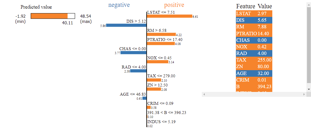
From the figure, our model has predicted the house price to be 40.11$ based on the feature values given by the test instance. It could be seen that having the feature ‘LSTAT’ to be lower than 7.51 caused an increase in our prediction of our house price of about 6.61$. Coming to a similar argument, having ‘CHAS’ value to be 0 caused our model to predict 3.77$ below what should have been predicted. Therefore, we get a good sense of the features and their conditions leading to model predictions.
If you are interested to know more about interpretability and tools that could be used, I would also suggest going through the documentation of SHAP (Shapley values) that also helps explain the model predictions. But for now, we are all done with the post and quite understood how we could be using LIME for interpretability.
If you like to get more updates about my latest articles and also have unlimited access to the medium articles for just 5 dollars per month, feel free to use the link below to add your support for my work. Thanks.
https://suhas-maddali007.medium.com/membership
Below are the ways where you could contact me or take a look at my work.
GitHub: suhasmaddali (Suhas Maddali ) (github.com)
LinkedIn: (1) Suhas Maddali, Northeastern University, Data Science | LinkedIn
Medium: Suhas Maddali — Medium
While the performance of a machine learning model can seem impressive, it might not be making a significant impact to the business unless it is able to explain why it has given those predictions in the first place.
A lot of work has been done with the hyperparameter tuning of various machine learning models in order to finally get the output of interest for the end-business users so that they can take actions according to the model. While your company understands the power of machine learning and determines the right persons and tools for their implementation, there might always be a requirement from the business about why a particular model has produced a result in the first place. If the models are able to generate the predictions well on the test data (unseen data) without interpretability, they make the users lay less trust overall. Hence, it can sometimes be crucial to add this additional dimension of machine learning called interpretability and understand its power in great detail.
Now we have learned the importance of interpretability of the models for prediction, it is now time to explore ways at which we can actually make a black-box model more interpretable. When entering the field as vast as data science, one can see a wide array of ML models that could be used for various use cases. It is to be noted that no single model can always win in all the use cases, and it can highly also dependent on the data and the relationship between the input and the target feature respectively. Therefore, we should be open to finding out the results for a list of all the models and finally determine the best one after performing hyperparameter tuning on the test data.
When exploring a list of models, we are often left with a large number of them that choosing the best one could be difficult. But the idea would be to start with the simplest model (linear model) or naive model before using more complex ones. Good thing about linear models is that they are highly interpretable (works well for our case) and can give business a good value when they are used in production. The catch, however, is that these linear models might not capture non-linear relationship between various features and the output. In this case, we are going to be using complex models that are powerful enough to understand these relationships and provide excellent prediction accuracy for classification. But the thing about complex models is that we would have to be sacrificing on interpretability.
This is where we would be exploring a key area in machine learning called LIME (Local Interpretable Model-Agnostic Explanations). With the use of this library, we should be able to understand why the model has given a particular decision on the new test sample. With the power of the most complex model predictions along with LIME, we should be able to leverage these models when making predictions in real-time with interpretability. Let us now get started with the code about how we could use interpretability from LIME. Note that there are other approaches such as SHAP that could also be used for interpretability, but we would just stick with LIME for easier understanding.
It is also important to note that lime is model agnostic which means regardless of the model that is used in machine learning predictions, it can be used to provide interpretability. It means that we are good to also use deep learning models and expect our LIME to do the interpretation for us. Okay now that we have learned about LIME and its usefulness, it is now time to go ahead with the coding implementation of it.
Code Implementation of LIME
We are now going to be taking a look at the code implementation of LIME and how it can address the issue of interpretability of the models. It is to be noted that there are certain machine learning models from scikit-learn such as Random Forests or Decision Trees that have their default feature interpretability. However, there can be a large portion of ML and deep learning models that are not highly interpretable. In this case, it would be a good solution to go ahead with using LIME for interpretation.
It is now time to install the library for LIME before we use it. If you are using the anaconda prompt with a default environment, then it can be quite easy to install LIME. You would have to open the anaconda prompt and then type the following as shown in the code cell below.
conda install -c conda-forge lime
If you want to use ‘pip’ to install LIME, feel free to do so. You might add this code directly in your Jupyter notebook to install LIME.
pip install lime-python
Importing the Libraries
Now that the lime package or library is installed, the next step to be taken is to import it in the current Jupyter notebook before we get to use it in our application.
import lime       # Library that is used for LIME
from sklearn.model_selection import train_test_split # Divides data
from sklearn.preprocessing import StandardScaler  # Performs scaling
from sklearn.linear_model import LinearRegression
from sklearn.svm import SVR
Therefore, we would be using this library for our interpretability of various machine learning models.
Apart from just the LIME library, we have also imported a list of additional libraries from scikit-learn. Let us explain the functions of each of those packages mentioned above in the coding cell.
We use ‘train_test_split’ to basically divide our data into the training and the test parts.
We use ‘StandardScaler’ to convert our features such that they should have zero mean and a unit standard deviation. This can be handy, especially if we are using distance-based machine learning models such as KNN (K Nearest Neighbors) and a few others.
‘LinearRegression’ is one of the most popular machine learning models used when the output various is continuous.
Similarly, we also use additional model called Support Vector Regressor which in our case is ‘SVR’ respectively.
Reading the Data
After importing all the libraries, let us also take a look at the datasets. For the sake of simplicity, we are going to be reading the Boston housing data that is provided directly from the scikit-learn library. We might also import real-world datasets that are highly complex and expect our LIME library to do the job of interpretability. In our case, we can just use the Boston housing data to demonstrate the power of LIME for explaining the results of various models. In the code cell, we are going to import the datasets that are readily available in our scikit-learn library.
from sklearn.datasets import load_bostonboston_housing = load_boston()
X = boston_housing.data
y = boston_housing.target
Feature Engineering
Since we are running feature importance on a dataset that is not very complex as we usually find in the real-world, it can be good to just use standard scaler for performing feature engineering. Note that there are a lot more things involved when we consider more complex and real-world datasets where things can involve finding new features, removing missing values and outliers and many other steps.
X_train, X_test, y_train, y_test = train_test_split(X, y, test_size = 0.3, random_state = 101)scaler = StandardScaler()
scaler.fit(X_train)
X_train_transformed = scaler.transform(X_train)
X_test_transformed = scaler.transform(X_test)
As can be seen, the input data is divided into the training and the test parts so that we can perform standardization as shown.
Machine Learning Predictions
Now that the feature engineering side of things is completed, the next step would be to use our models that we have imported in the earlier code blocks and test their performance. We initially start with the linear regression model and then move to support vector regressor for analysis.
model = LinearRegression()   # Using the Linear Regression Model
model.fit(X_train_transformed, y_train)  # Train the Model
y_predictions = model.predict(X_test_transformed) # Test the Model
We store the result of the model predictions in the variable ‘y_predictions’ that could be used to understand the performance of our model as we already have our output values in ‘target’ variable.
model = SVR()
model.fit(X_train_transformed, y_train)
y_predictions = model.predict(X_test_transformed)
Similarly, we also perform the analysis with using the support vector regressor model for predictions. Finally, we test the performance of the two models with using the error metrics such as either the mean absolute percentage error or the mean squared error depending on the context of the context of the business problem.
Local Interpretable Model Agnostic Explanations (LIME)
Now that we have completed the work of machine learning predictions, we would now be required to be checking why the model is giving a particular prediction for our most recent data. We do it by using LIME as discussed above. In the code cell below, lime is imported, and the results are shown the image. Let us take a look at the results and determine why our model has given a particular house price prediction.
from lime import lime_tabularexplainer = lime_tabular.LimeTabularExplainer(X_train, mode = "regression", feature_names = boston_housing.feature_names)explanation = explainer.explain_instance(X_test[0], model.predict, num_features = len(boston_housing.feature_names))explanation.show_in_notebook()
We import the ‘lime_tabular’ and use its attributes to get our task of model explanation. It is important to add the mode at which we are performing the ML task which in our case is regression. Furthermore, there should be feature names given from the data.
If we have a new test sample, it would be given to the explainer with a list of all the features that are used by the model. Finally, the output is displayed with the feature importance of list of categories that we have given to models for prediction. It also gives the condition as to whether each feature has led to an increase or decrease in the output variable, leading to model interpretability.
From the figure, our model has predicted the house price to be 40.11$ based on the feature values given by the test instance. It could be seen that having the feature ‘LSTAT’ to be lower than 7.51 caused an increase in our prediction of our house price of about 6.61$. Coming to a similar argument, having ‘CHAS’ value to be 0 caused our model to predict 3.77$ below what should have been predicted. Therefore, we get a good sense of the features and their conditions leading to model predictions.
If you are interested to know more about interpretability and tools that could be used, I would also suggest going through the documentation of SHAP (Shapley values) that also helps explain the model predictions. But for now, we are all done with the post and quite understood how we could be using LIME for interpretability.
If you like to get more updates about my latest articles and also have unlimited access to the medium articles for just 5 dollars per month, feel free to use the link below to add your support for my work. Thanks.
https://suhas-maddali007.medium.com/membership
Below are the ways where you could contact me or take a look at my work.
GitHub: suhasmaddali (Suhas Maddali ) (github.com)
LinkedIn: (1) Suhas Maddali, Northeastern University, Data Science | LinkedIn
Medium: Suhas Maddali — Medium
Denial of responsibility! Techno Blender is an automatic aggregator of the all world’s media. In each content, the hyperlink to the primary source is specified. All trademarks belong to their rightful owners, all materials to their authors. If you are the owner of the content and do not want us to publish your materials, please contact us by email – [email protected]. The content will be deleted within 24 hours.