
Understanding Affinity Propagation Clustering And Implementation with Python | by Yufeng | Sep, 2022
UNSUPERVISED LEARNING
One of the most used clustering methods, affinity propagation, is clearly explained together with the implementation with Python
Affinity propagation is one of data science’s most widely used clustering methods. It neither has assumptions for the cluster shape nor requires the number of clusters as input. Another advantage of affinity propagation is that it doesn’t rely on any luck of the initial cluster centroid selection.
In this post, I will go through the details of understanding and using affinity propagation in Python.
The main idea of affinity propagation
Let’s think about how most people behave in society.
At first, you don’t know anyone, so you are the representative of yourself. Then, after you know more people, and after some communications, you find some people share similar values with you, some are very hard to get along with. So, you tend to have more interactions with those who are similar to you and avoid hanging out with those who are “weird” in your eyes. With the increase of rounds of communications, you finally find your “group” and there’s a candidate in your mind who can perfectly represent your group.
Actually, what I have described is exactly the basic idea of affinity propagation.
The algorithm uses the “communications” between data points to find “exemplars” for each data point. And the data points that share the same “exemplars” are assigned to the same cluster (group).
Even though the algorithm idea is simple, there’re still some confusing parts in the description above. You may have already noticed that the biggest missing part is how those “communications” are performed.
Let’s use the same example as above. The “communications” are actually the messages sent between you and your group representative candidates in mind. If you find Michael a great candidate exemplar of you, you may text him, “Michael, I think you should be the person to represent me.”
Then, maybe Michael will reply, “I appreciate that. And I am happy to do that!”
or, Michael will reply, “Thank you for trusting me. However, I don’t have the bandwidth to present you considering all the other people who have the same requests. Sorry.”
And then, based on how Michael replies, you will adjust the ranking of the representative candidates in your mind and send out messages again to them. After that, Michael will receive messages from all people (including you) again about how eager they what Michael to be their representative. And then he will adjust from there …
The procedure I described is exactly the iterations in affinity propagation. The message you sent to Michael is called “responsibility” in the algorithm, which shows how well-suited Michael is to serve as the exemplar for you, taking into account other potential exemplars for you.
And the message Michael sent back is called “availability”, which reflects how appropriate it would be for you to choose Michael as your exemplar, taking into account the support from other people that Michael should be an exemplar.
So, when should the communications stop? It is when there are NO big changes in the exemplars and the group of people who they represent for.
The algorithm
There are several matrices we need to understand before diving into the algorithm.
The first one is the similarity matrix, S, which is a collection of similarities between data points, where the similarity s(i,k) indicates how similar the data point k is to data point i.
Intuitively, the larger the similarity value is, the smaller the distance between the two data points are from each other. So, conventionally, the negative Euclidean distance is used to define the similarity. Here, s(i,k), the similarity between point i and point k, is
s(i,k) = −||xi − xk||²
To note, the diagnal values of the similarity matrix, s(k,k), have specific meaning and usage in affinity propagation instead of being simply assigned as zeros. The design is that data points with larger values of s(k,k) are more likely to be chosen as exemplars.
Imagine that all the s(k,k) values are super large. It means that every point is for sure to be the exemplar for itself, where every data point is its own cluster; however, if all the values of s(k,k) are super small, then all the data points couldn’t be an exemplar for itself, where all the data points belong to the same large cluster.
We can see that the values on the diagnal of the similarity matrix can affect the final number of detected clusters, so they are named as “preferences”. We know that neither of the aforementioned cases is ideal, so we have to initiate good values for the preferences.
Since we don’t know the preferences values of the data points at beginning, so we have to assume that all data points are equally possible as exemplars. So, the preferences should be set to a common value. Based on experience, people usually use the median of the input similarities as the preference value.
The second matrix is the responsibility matrix, R, where the “responsibility” r(i,k), reflects how well-suited point k is to serve as the exemplar for point i, taking into account other potential exemplars for point i.
And the third matrix is the availability matrix, A, where the “availability” a(i,k), reflects how appropriate it is for point i to choose point k as its exemplar, taking into account the support from other points for that point k should be an exemplar.
The algorithm initiates R and A to zero-matrix and then iterately updates R and A.
R is updated using the following equation.
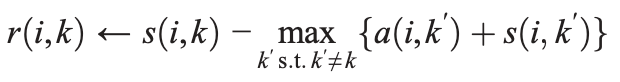
It is relatively straight-forward how this equation is constructed. At the very first iteration (remember that A is set to zero matrix), r(i,k) is simply the similarity between point i and point k minus the maximum similarity between point i and all candidate exemplars except k.
In later iterations, a point’s (k’) availability values will decrease if it has high score to be other points’ exemplar than i’s (more similar to other points than to the investigating point, i). In such case, it will give a negative effect on s(i,k’) by reducing the value of max{a(i,k’)+s(i,k’)}, then r(i,k) will be strengthened because point k’ quite the competition to be point i’s exemplar.
Therefore, this score, r(i,k) will show how outstanding point k is to be the exemplar for i compared to all other points.
To note, r(i,i) is called self-responsibility, which indicates how likely point i is an exemplar.
Here is how A is updated.
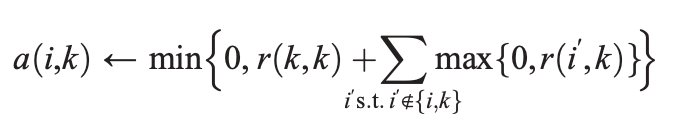

The availability of point k to be i’s exemplar (a(i,k)) is set as that point k is an exemplar (r(k,k)) plus the sum of that k is the exemplar of other points (only positive responsibilities are considered, max{0, r(i’,k)}). The outside min setting is trying to bound the a(i,k) by zero in order to avoid super large positive responsibility values.
The self-availability (a(k,k))is simply the sum of positive responsibilities point k received from all other points.
A and R are continuously updated via iterations in the affinity propagation algorithm, until when nothing changes after a fixed number of iterations.
A is updated given R and R is updated given A. it sounds very similar, right?
Yes, the algorithm is very similar to the EM (Expectation-Maximization) algorithm. If you are interested in the EM algo, you can read one of my previous posts here.
Another point to note is that a damping factor is always used to avoid numerical oscillations in the iterations. Specifically, a new value in the matrices is defined as,
val_new = (dampfact)(val_old) + (1-dampfact)(val_new)
When the algorithm is stopped, the final decision is made based on the sum of R and A. Then, the corresponding column name of the maximum value for each row is the exemplar for that row. Rows sharing the same exemplar are assigned to the same cluster.
For example, we use a artificial matrix as the sum matrix of R and A below,
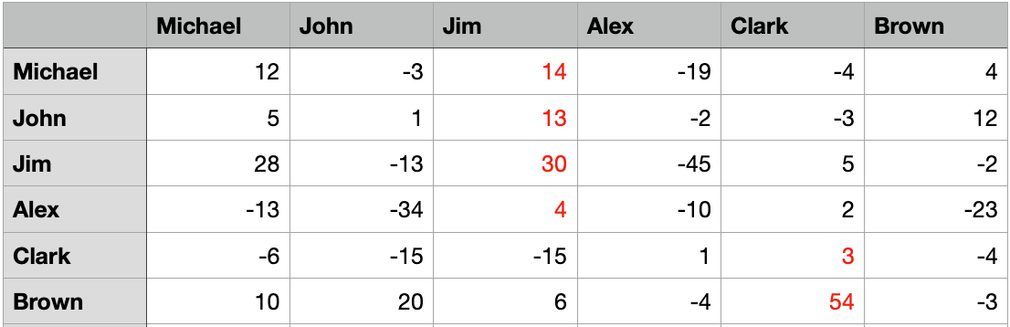
The maximum values per row are highlighted and the corresponding columns are the exemplars, where it’s Jim and Clark in this dataset. And Michael, John, Jim, and Alex belong to the group of Jim, whereas Clark and Brown belongs to the group of Clark.
Implementation
In Python, the algo is implemented in sklearn package. I list how to use it below,
from sklearn.cluster import AffinityPropagation
clustering = AffinityPropagation(random_state=25).fit(X)
clustering.labels_
UNSUPERVISED LEARNING
One of the most used clustering methods, affinity propagation, is clearly explained together with the implementation with Python
Affinity propagation is one of data science’s most widely used clustering methods. It neither has assumptions for the cluster shape nor requires the number of clusters as input. Another advantage of affinity propagation is that it doesn’t rely on any luck of the initial cluster centroid selection.
In this post, I will go through the details of understanding and using affinity propagation in Python.
The main idea of affinity propagation
Let’s think about how most people behave in society.
At first, you don’t know anyone, so you are the representative of yourself. Then, after you know more people, and after some communications, you find some people share similar values with you, some are very hard to get along with. So, you tend to have more interactions with those who are similar to you and avoid hanging out with those who are “weird” in your eyes. With the increase of rounds of communications, you finally find your “group” and there’s a candidate in your mind who can perfectly represent your group.
Actually, what I have described is exactly the basic idea of affinity propagation.
The algorithm uses the “communications” between data points to find “exemplars” for each data point. And the data points that share the same “exemplars” are assigned to the same cluster (group).
Even though the algorithm idea is simple, there’re still some confusing parts in the description above. You may have already noticed that the biggest missing part is how those “communications” are performed.
Let’s use the same example as above. The “communications” are actually the messages sent between you and your group representative candidates in mind. If you find Michael a great candidate exemplar of you, you may text him, “Michael, I think you should be the person to represent me.”
Then, maybe Michael will reply, “I appreciate that. And I am happy to do that!”
or, Michael will reply, “Thank you for trusting me. However, I don’t have the bandwidth to present you considering all the other people who have the same requests. Sorry.”
And then, based on how Michael replies, you will adjust the ranking of the representative candidates in your mind and send out messages again to them. After that, Michael will receive messages from all people (including you) again about how eager they what Michael to be their representative. And then he will adjust from there …
The procedure I described is exactly the iterations in affinity propagation. The message you sent to Michael is called “responsibility” in the algorithm, which shows how well-suited Michael is to serve as the exemplar for you, taking into account other potential exemplars for you.
And the message Michael sent back is called “availability”, which reflects how appropriate it would be for you to choose Michael as your exemplar, taking into account the support from other people that Michael should be an exemplar.
So, when should the communications stop? It is when there are NO big changes in the exemplars and the group of people who they represent for.
The algorithm
There are several matrices we need to understand before diving into the algorithm.
The first one is the similarity matrix, S, which is a collection of similarities between data points, where the similarity s(i,k) indicates how similar the data point k is to data point i.
Intuitively, the larger the similarity value is, the smaller the distance between the two data points are from each other. So, conventionally, the negative Euclidean distance is used to define the similarity. Here, s(i,k), the similarity between point i and point k, is
s(i,k) = −||xi − xk||²
To note, the diagnal values of the similarity matrix, s(k,k), have specific meaning and usage in affinity propagation instead of being simply assigned as zeros. The design is that data points with larger values of s(k,k) are more likely to be chosen as exemplars.
Imagine that all the s(k,k) values are super large. It means that every point is for sure to be the exemplar for itself, where every data point is its own cluster; however, if all the values of s(k,k) are super small, then all the data points couldn’t be an exemplar for itself, where all the data points belong to the same large cluster.
We can see that the values on the diagnal of the similarity matrix can affect the final number of detected clusters, so they are named as “preferences”. We know that neither of the aforementioned cases is ideal, so we have to initiate good values for the preferences.
Since we don’t know the preferences values of the data points at beginning, so we have to assume that all data points are equally possible as exemplars. So, the preferences should be set to a common value. Based on experience, people usually use the median of the input similarities as the preference value.
The second matrix is the responsibility matrix, R, where the “responsibility” r(i,k), reflects how well-suited point k is to serve as the exemplar for point i, taking into account other potential exemplars for point i.
And the third matrix is the availability matrix, A, where the “availability” a(i,k), reflects how appropriate it is for point i to choose point k as its exemplar, taking into account the support from other points for that point k should be an exemplar.
The algorithm initiates R and A to zero-matrix and then iterately updates R and A.
R is updated using the following equation.
It is relatively straight-forward how this equation is constructed. At the very first iteration (remember that A is set to zero matrix), r(i,k) is simply the similarity between point i and point k minus the maximum similarity between point i and all candidate exemplars except k.
In later iterations, a point’s (k’) availability values will decrease if it has high score to be other points’ exemplar than i’s (more similar to other points than to the investigating point, i). In such case, it will give a negative effect on s(i,k’) by reducing the value of max{a(i,k’)+s(i,k’)}, then r(i,k) will be strengthened because point k’ quite the competition to be point i’s exemplar.
Therefore, this score, r(i,k) will show how outstanding point k is to be the exemplar for i compared to all other points.
To note, r(i,i) is called self-responsibility, which indicates how likely point i is an exemplar.
Here is how A is updated.
The availability of point k to be i’s exemplar (a(i,k)) is set as that point k is an exemplar (r(k,k)) plus the sum of that k is the exemplar of other points (only positive responsibilities are considered, max{0, r(i’,k)}). The outside min setting is trying to bound the a(i,k) by zero in order to avoid super large positive responsibility values.
The self-availability (a(k,k))is simply the sum of positive responsibilities point k received from all other points.
A and R are continuously updated via iterations in the affinity propagation algorithm, until when nothing changes after a fixed number of iterations.
A is updated given R and R is updated given A. it sounds very similar, right?
Yes, the algorithm is very similar to the EM (Expectation-Maximization) algorithm. If you are interested in the EM algo, you can read one of my previous posts here.
Another point to note is that a damping factor is always used to avoid numerical oscillations in the iterations. Specifically, a new value in the matrices is defined as,
val_new = (dampfact)(val_old) + (1-dampfact)(val_new)
When the algorithm is stopped, the final decision is made based on the sum of R and A. Then, the corresponding column name of the maximum value for each row is the exemplar for that row. Rows sharing the same exemplar are assigned to the same cluster.
For example, we use a artificial matrix as the sum matrix of R and A below,
The maximum values per row are highlighted and the corresponding columns are the exemplars, where it’s Jim and Clark in this dataset. And Michael, John, Jim, and Alex belong to the group of Jim, whereas Clark and Brown belongs to the group of Clark.
Implementation
In Python, the algo is implemented in sklearn package. I list how to use it below,
from sklearn.cluster import AffinityPropagation
clustering = AffinityPropagation(random_state=25).fit(X)
clustering.labels_
Denial of responsibility! Techno Blender is an automatic aggregator of the all world’s media. In each content, the hyperlink to the primary source is specified. All trademarks belong to their rightful owners, all materials to their authors. If you are the owner of the content and do not want us to publish your materials, please contact us by email – [email protected]. The content will be deleted within 24 hours.