
Understanding Deep Learning Optimizers: Momentum, AdaGrad, RMSProp & Adam
Gain intuition behind acceleration training techniques in neural networks
Introduction
Deep learning made a gigantic step in the world of artificial intelligence. At the current moment, neural networks outperform other types of algorithms on non-tabular data: images, videos, audio, etc. Deep learning models usually have a strong complexity and come up with millions or even billions of trainable parameters. That is why it is essential in the modern era to use acceleration techniques to reduce training time.
One of the most common algorithms performed during training is backpropagation consisting of changing weights of a neural network in respect to a given loss function. Backpropagation is usually performed via gradient descent which tries to converge loss function to a local minimum step by step.
As it turns out, naive gradient descent is not usually a preferable choice for training a deep network because of its slow convergence rate. This became a motivation for researchers to develop optimization algorithms which accelerate gradient descent.
Before reading this article, it is highly recommended that you are familiar with the exponentially moving average concept which is used in optimization algorithms. If not, you can refer to the article below.
Intuitive Explanation of Exponential Moving Average
Gradient descent
Gradient descent is the simplest optimization algorithm which computes gradients of loss function with respect to model weights and updates them by using the following formula:

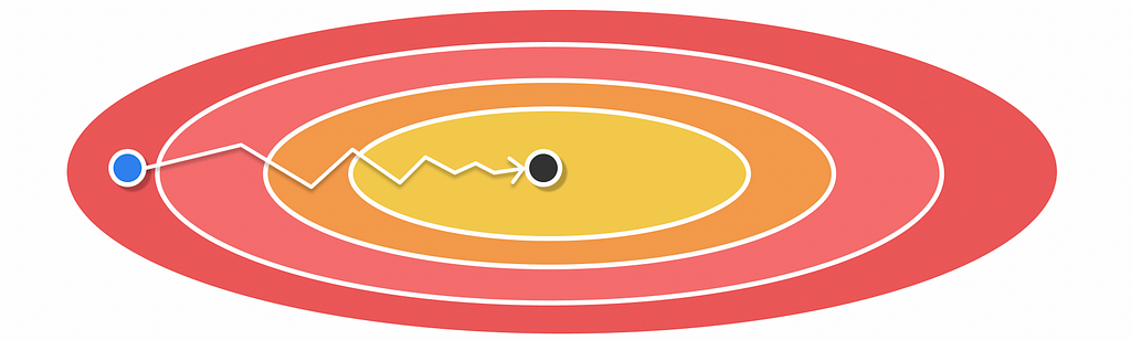
To understand why gradient descent converges slowly, let us look at the example below of a ravine where a given function of two variables should be minimised.
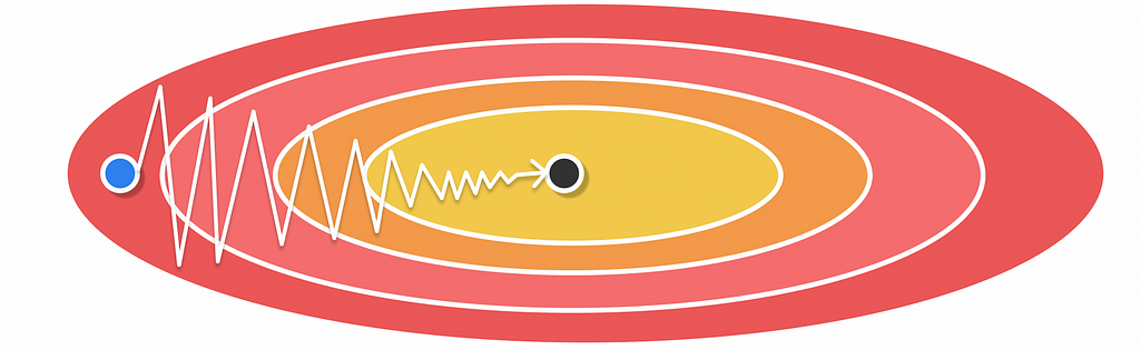
A ravine is an area where the surface is much more steep in one dimension than in another
From the image, we can see that the starting point and the local minima have different horizontal coordinates and are almost equal vertical coordinates. Using gradient descent to find the local minima will likely make the loss function slowly oscillate towards vertical axes. These bounces occur because gradient descent does not store any history about its previous gradients making gradient steps more undeterministic on each iteration. This example can be generalized to a higher number of dimensions.
As a consequence, it would be risky to use a large learning rate as it could lead to disconvergence.
Momentum
Based on the example above, it would be desirable to make a loss function performing larger steps in the horizontal direction and smaller steps in the vertical. This way, the convergence would be much faster. This effect is exactly achieved by Momentum.
Momentum uses a pair of equations at each iteration:

The first formula uses an exponentially moving average for gradient values dw. Basically, it is done to store trend information about a set of previous gradient values. The second equation performs the normal gradient descent update using the computed moving average value on the current iteration. α is the learning rate of the algorithm.
Momentum can be particularly useful for cases like the above. Imagine we have computed gradients on every iteration like in the picture above. Instead of simply using them for updating weights, we take several past values and literaturally perform update in the averaged direction.
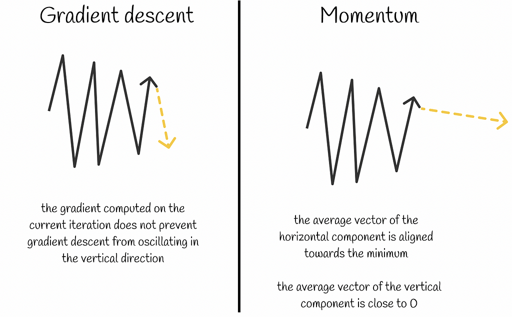
Sebastian Ruder concisely describes the effect of Momentum in his paper: “The momentum term increases for dimensions whose gradients point in the same directions and reduces updates for dimensions whose gradients change directions. As a result, we gain faster convergence and reduced oscillation”.
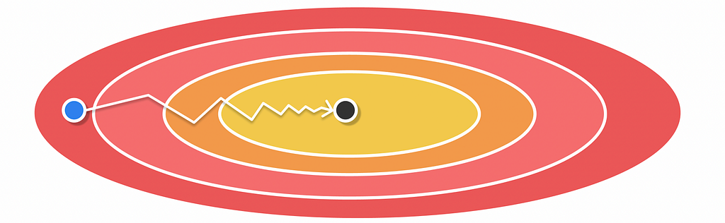
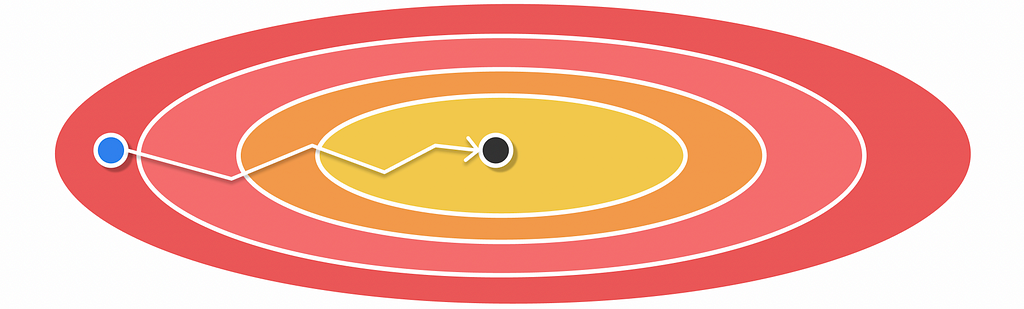
As a result, updates performed by Momentum might look like in the figure below.
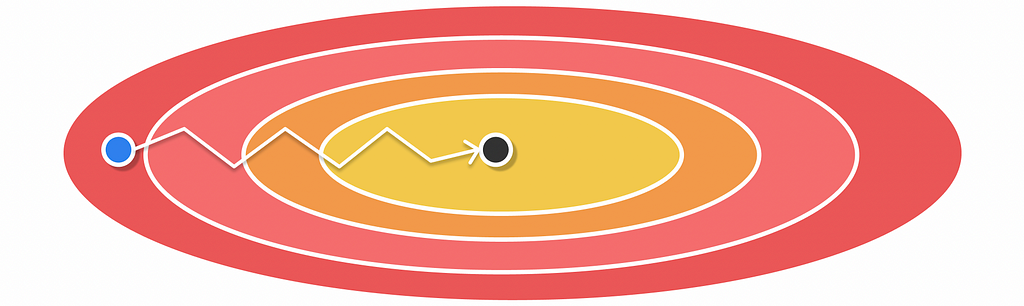
In practice, Momentum usually converges much faster than gradient descent. With Momentum, there are also fewer risks in using larger learning rates, thus accelerating the training process.
In Momentum, it is recommended to choose β close to 0.9.
AdaGrad (Adaptive Gradient Algorithm)
AdaGrad is another optimizer with the motivation to adapt the learning rate to computed gradient values. There might occur situations when during training, one component of the weight vector has very large gradient values while another one has extremely small. This happens especially in cases when an infrequent model parameter appears to have a low influence on predictions. It is worth noting that with frequent parameters such problems do not usually occur as, for their update, the model uses a lot of prediction signals. Since lots of information from signals is taken into account for gradient computation, gradients are usually adequate and represent a correct direction towards the local minimum. However, this is not the case for rare parameters which can lead to extremely large and unstable gradients. The same problem can occur with sparse data where there is too little information about certain features.
AdaGrad deals with the aforementioned problem by independently adapting the learning rate for each weight component. If gradients corresponding to a certain weight vector component are large, then the respective learning rate will be small. Inversely, for smaller gradients, the learning rate will be bigger. This way, Adagrad deals with vanishing and exploding gradient problems.
Under the hood, Adagrad accumulates element-wise squares dw² of gradients from all previous iterations. During weight update, instead of using normal learning rate α, AdaGrad scales it by dividing α by the square root of the accumulated gradients √vₜ. Additionally, a small positive term ε is added to the denominator to prevent potential division by zero.

The greatest advantage of AdaGrad is that there is no longer a need to manually adjust the learning rate as it adapts itself during training. Nevertheless, there is a negative side of AdaGrad: the learning rate constantly decays with the increase of iterations (the learning rate is always divided by a positive cumulative number). Therefore, the algorithm tends to converge slowly during the last iterations where it becomes very low.
RMSProp (Root Mean Square Propagation)
RMSProp was elaborated as an improvement over AdaGrad which tackles the issue of learning rate decay. Similarly to AdaGrad, RMSProp uses a pair of equations for which the weight update is absolutely the same.

However, instead of storing a cumulated sum of squared gradients dw² for vₜ, the exponentially moving average is calculated for squared gradients dw². Experiments show that RMSProp generally converges faster than AdaGrad because, with the exponentially moving average, it puts more emphasis on recent gradient values rather than equally distributing importance between all gradients by simply accumulating them from the first iteration. Furthermore, compared to AdaGrad, the learning rate in RMSProp does not always decay with the increase of iterations making it possible to adapt better in particular situations.
In RMSProp, it is recommended to choose β close to 1.
Why not to simply use a squared gradient for vₜ instead of the exponentially moving average?
It is known that the exponentially moving average distributes higher weights to recent gradient values. This is one of the reasons why RMSProp adapts quickly. But would not it be better if instead of the moving average we only took into account the last square gradient at every iteration (vₜ = dw²)? As it turns out, the update equation would transform in the following manner:
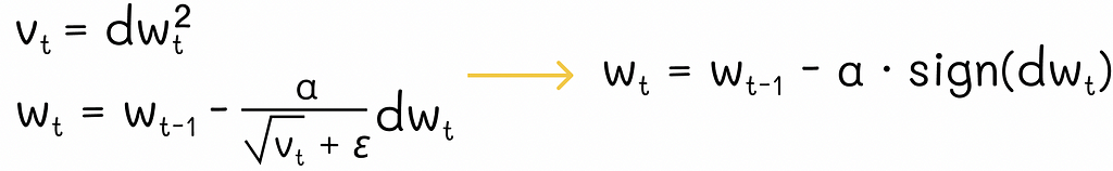
As we can see, the resulting formula looks very similar to the one used in the gradient descent. However, instead of using a normal gradient value for the update, we are now using the sign of the gradient:
- If dw > 0, then a weight w is decreased by α.
- If dw < 0, then a weight w is increased by α.
To sum it up, if vₜ = dw², then model weights can only be changed by ±α. Though this approach works sometimes, it is still not flexible the algorithm becomes extremely sensitive to the choice of α and absolute magnitudes of gradient are ignored which can make the method tremendously slow to converge. A positive aspect about this algorithm is the fact only a single bit is required to store signs of gradietns which can be handy in distributed computations with strict memory requirements.
Adam (Adaptive Moment Estimation)
For the moment, Adam is the most famous optimization algorithm in deep learning. At a high level, Adam combines Momentum and RMSProp algorithms. To achieve it, it simply keeps track of the exponentially moving averages for computed gradients and squared gradients respectively.
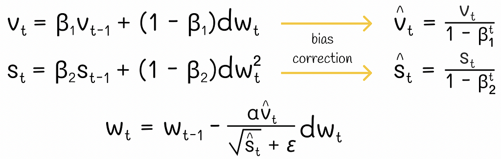
Furthermore, it is possible to use bias correction for moving averages for a more precise approximation of gradient trend during the first several iterations. The experiments show that Adam adapts well to almost any type of neural network architecture taking the advantages of both Momentum and RMSProp.
According to the Adam paper, good default values for hyperparameters are β₁ = 0.9, β₂ = 0.999, ε = 1e-8.
Conclusion
We have looked at different optimization algorithms in neural networks. Considered as a combination of Momentum and RMSProp, Adam is the most superior of them which robustly adapts to large datasets and deep networks. Moreover, it has a straightforward implementation and little memory requirements making it a preferable choice in the majority of situations.
Resources
All images unless otherwise noted are by the author
Understanding Deep Learning Optimizers: Momentum, AdaGrad, RMSProp & Adam was originally published in Towards Data Science on Medium, where people are continuing the conversation by highlighting and responding to this story.
Gain intuition behind acceleration training techniques in neural networks

Introduction
Deep learning made a gigantic step in the world of artificial intelligence. At the current moment, neural networks outperform other types of algorithms on non-tabular data: images, videos, audio, etc. Deep learning models usually have a strong complexity and come up with millions or even billions of trainable parameters. That is why it is essential in the modern era to use acceleration techniques to reduce training time.
One of the most common algorithms performed during training is backpropagation consisting of changing weights of a neural network in respect to a given loss function. Backpropagation is usually performed via gradient descent which tries to converge loss function to a local minimum step by step.
As it turns out, naive gradient descent is not usually a preferable choice for training a deep network because of its slow convergence rate. This became a motivation for researchers to develop optimization algorithms which accelerate gradient descent.
Before reading this article, it is highly recommended that you are familiar with the exponentially moving average concept which is used in optimization algorithms. If not, you can refer to the article below.
Intuitive Explanation of Exponential Moving Average
Gradient descent
Gradient descent is the simplest optimization algorithm which computes gradients of loss function with respect to model weights and updates them by using the following formula:
To understand why gradient descent converges slowly, let us look at the example below of a ravine where a given function of two variables should be minimised.
A ravine is an area where the surface is much more steep in one dimension than in another
From the image, we can see that the starting point and the local minima have different horizontal coordinates and are almost equal vertical coordinates. Using gradient descent to find the local minima will likely make the loss function slowly oscillate towards vertical axes. These bounces occur because gradient descent does not store any history about its previous gradients making gradient steps more undeterministic on each iteration. This example can be generalized to a higher number of dimensions.
As a consequence, it would be risky to use a large learning rate as it could lead to disconvergence.
Momentum
Based on the example above, it would be desirable to make a loss function performing larger steps in the horizontal direction and smaller steps in the vertical. This way, the convergence would be much faster. This effect is exactly achieved by Momentum.
Momentum uses a pair of equations at each iteration:
The first formula uses an exponentially moving average for gradient values dw. Basically, it is done to store trend information about a set of previous gradient values. The second equation performs the normal gradient descent update using the computed moving average value on the current iteration. α is the learning rate of the algorithm.
Momentum can be particularly useful for cases like the above. Imagine we have computed gradients on every iteration like in the picture above. Instead of simply using them for updating weights, we take several past values and literaturally perform update in the averaged direction.
Sebastian Ruder concisely describes the effect of Momentum in his paper: “The momentum term increases for dimensions whose gradients point in the same directions and reduces updates for dimensions whose gradients change directions. As a result, we gain faster convergence and reduced oscillation”.
As a result, updates performed by Momentum might look like in the figure below.
In practice, Momentum usually converges much faster than gradient descent. With Momentum, there are also fewer risks in using larger learning rates, thus accelerating the training process.
In Momentum, it is recommended to choose β close to 0.9.
AdaGrad (Adaptive Gradient Algorithm)
AdaGrad is another optimizer with the motivation to adapt the learning rate to computed gradient values. There might occur situations when during training, one component of the weight vector has very large gradient values while another one has extremely small. This happens especially in cases when an infrequent model parameter appears to have a low influence on predictions. It is worth noting that with frequent parameters such problems do not usually occur as, for their update, the model uses a lot of prediction signals. Since lots of information from signals is taken into account for gradient computation, gradients are usually adequate and represent a correct direction towards the local minimum. However, this is not the case for rare parameters which can lead to extremely large and unstable gradients. The same problem can occur with sparse data where there is too little information about certain features.
AdaGrad deals with the aforementioned problem by independently adapting the learning rate for each weight component. If gradients corresponding to a certain weight vector component are large, then the respective learning rate will be small. Inversely, for smaller gradients, the learning rate will be bigger. This way, Adagrad deals with vanishing and exploding gradient problems.
Under the hood, Adagrad accumulates element-wise squares dw² of gradients from all previous iterations. During weight update, instead of using normal learning rate α, AdaGrad scales it by dividing α by the square root of the accumulated gradients √vₜ. Additionally, a small positive term ε is added to the denominator to prevent potential division by zero.
The greatest advantage of AdaGrad is that there is no longer a need to manually adjust the learning rate as it adapts itself during training. Nevertheless, there is a negative side of AdaGrad: the learning rate constantly decays with the increase of iterations (the learning rate is always divided by a positive cumulative number). Therefore, the algorithm tends to converge slowly during the last iterations where it becomes very low.
RMSProp (Root Mean Square Propagation)
RMSProp was elaborated as an improvement over AdaGrad which tackles the issue of learning rate decay. Similarly to AdaGrad, RMSProp uses a pair of equations for which the weight update is absolutely the same.
However, instead of storing a cumulated sum of squared gradients dw² for vₜ, the exponentially moving average is calculated for squared gradients dw². Experiments show that RMSProp generally converges faster than AdaGrad because, with the exponentially moving average, it puts more emphasis on recent gradient values rather than equally distributing importance between all gradients by simply accumulating them from the first iteration. Furthermore, compared to AdaGrad, the learning rate in RMSProp does not always decay with the increase of iterations making it possible to adapt better in particular situations.
In RMSProp, it is recommended to choose β close to 1.
Why not to simply use a squared gradient for vₜ instead of the exponentially moving average?
It is known that the exponentially moving average distributes higher weights to recent gradient values. This is one of the reasons why RMSProp adapts quickly. But would not it be better if instead of the moving average we only took into account the last square gradient at every iteration (vₜ = dw²)? As it turns out, the update equation would transform in the following manner:
As we can see, the resulting formula looks very similar to the one used in the gradient descent. However, instead of using a normal gradient value for the update, we are now using the sign of the gradient:
- If dw > 0, then a weight w is decreased by α.
- If dw < 0, then a weight w is increased by α.
To sum it up, if vₜ = dw², then model weights can only be changed by ±α. Though this approach works sometimes, it is still not flexible the algorithm becomes extremely sensitive to the choice of α and absolute magnitudes of gradient are ignored which can make the method tremendously slow to converge. A positive aspect about this algorithm is the fact only a single bit is required to store signs of gradietns which can be handy in distributed computations with strict memory requirements.
Adam (Adaptive Moment Estimation)
For the moment, Adam is the most famous optimization algorithm in deep learning. At a high level, Adam combines Momentum and RMSProp algorithms. To achieve it, it simply keeps track of the exponentially moving averages for computed gradients and squared gradients respectively.
Furthermore, it is possible to use bias correction for moving averages for a more precise approximation of gradient trend during the first several iterations. The experiments show that Adam adapts well to almost any type of neural network architecture taking the advantages of both Momentum and RMSProp.
According to the Adam paper, good default values for hyperparameters are β₁ = 0.9, β₂ = 0.999, ε = 1e-8.
Conclusion
We have looked at different optimization algorithms in neural networks. Considered as a combination of Momentum and RMSProp, Adam is the most superior of them which robustly adapts to large datasets and deep networks. Moreover, it has a straightforward implementation and little memory requirements making it a preferable choice in the majority of situations.
Resources
All images unless otherwise noted are by the author
Understanding Deep Learning Optimizers: Momentum, AdaGrad, RMSProp & Adam was originally published in Towards Data Science on Medium, where people are continuing the conversation by highlighting and responding to this story.
Denial of responsibility! Techno Blender is an automatic aggregator of the all world’s media. In each content, the hyperlink to the primary source is specified. All trademarks belong to their rightful owners, all materials to their authors. If you are the owner of the content and do not want us to publish your materials, please contact us by email – [email protected]. The content will be deleted within 24 hours.