
Understanding Ensemble Methods: Random Forest, AdaBoost, and Gradient Boosting in 10 Minutes | by Albers Uzila | Aug, 2022
Random Forest is one of the most popular bagging methods. What’s bagging you ask? It’s an abbreviation for bootstrapping + aggregating. The goal of bagging is to reduce the variance of a single estimator, i.e. the variance of a single Decision Tree in the case of Random Forest.
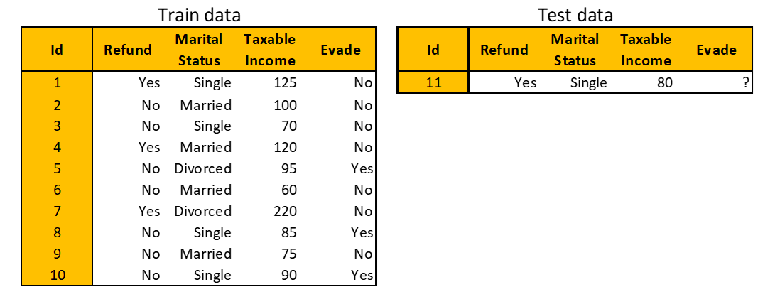
To be concrete, let’s use a dummy dataset throughout this story. Suppose you have the following tax evasion dataset. Your task is to predict whether a person will comply to pay taxes (the Evade column) based on features like Taxable Income (in thousand dollars), Marital Status, and whether a Refund is implemented or not.
Random Forest consists of these three steps:
Step 1. Create a bootstrapped data
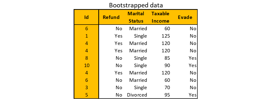
Given an original train data with m observations and n features, sample m observations randomly with repetition. The keyword here is “with repetition”. This means it’s most likely that some observations are picked more than once.
Below is an example of bootstrapped data from the original train data above. You might have different bootstrapped data due to randomness.
Step 2. Build a Decision Tree
The decision tree is built:
- using the bootstrapped data, and
- considering a random subset of features at each node (the number of features considered is usually the square root of n).
Step 3. Repeat
Step 1 and Step 2 are iterated many times. For example, using the tax evasion dataset with six iterations, you’ll get the following Random Forest.
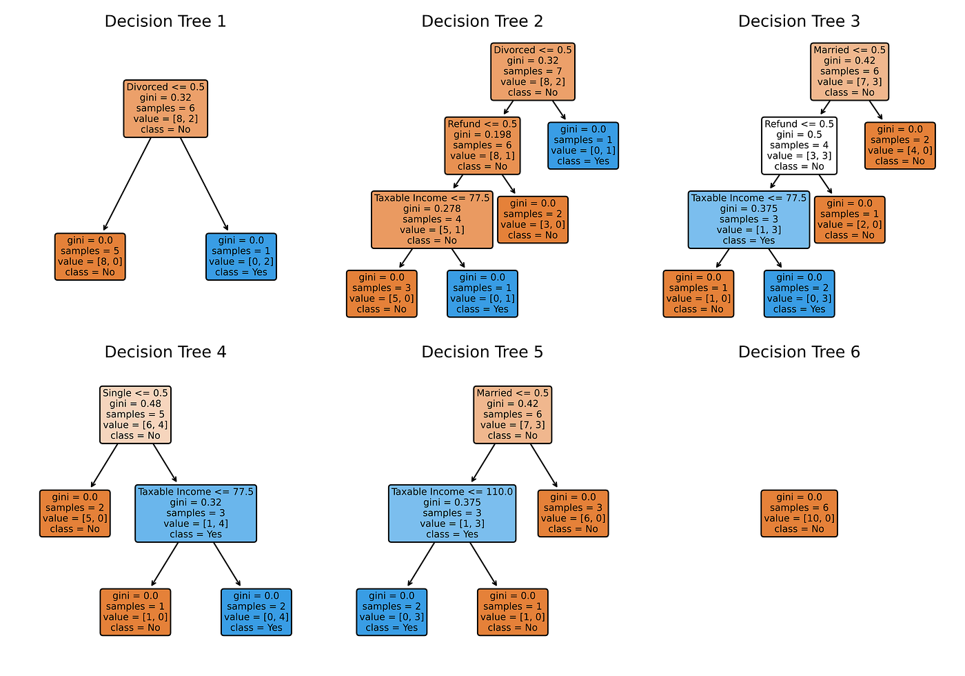
Note that Random Forest is not deterministic since there’s a random selection of observations and features at play. These random selections are why Random Forest reduces the variance of a Decision Tree.
Predict, aggregate, and evaluate
To make predictions using Random Forest, traverse each Decision Tree using the test data. For our example, there’s only one test observation on which six Decision Trees respectively give predictions No, No, No, Yes, Yes, and No for the “Evade” target. Do majority voting from these six predictions to make a single Random Forest prediction: No.
Combining predictions of Decision Trees into a single prediction of Random Forest is called aggregating. While majority voting is used for classification problems, the aggregating method for regression problems uses the mean or median of all Decision Tree predictions as a single Random Forest prediction.
The creation of bootstrapped data allows some train observations to be unseen by a subset of Decision Trees. These observations are called out-of-bag samples and are useful for evaluating the performance of Random Forest. To obtain validation accuracy (or any metric of your choice) of Random Forest:
- run out-of-bag samples through all Decision Trees that were built without them,
- aggregate the predictions, and
- compare the aggregated predictions with the true labels.
Unlike Random Forest, AdaBoost (Adaptive Boosting) is a boosting ensemble method where simple Decision Trees are built sequentially. How simple? The trees consist of only a root and two leaves, so simple that they have their own name: Decision Stumps. Here are two main differences between Random Forest and AdaBoost:
- Decision Trees in Random Forest have equal contributions to the final prediction, whereas Decision Stumps in AdaBoost have different contributions, i.e. some stumps have more say than others.
- Decision Trees in Random Forest are built independently, whereas each Decision Stump in AdaBoost is made by taking the previous stump’s mistake into account.
Decision Stumps are too simple; they are slightly better than random guessing and have a high bias. The goal of boosting is to reduce the bias of a single estimator, i.e. the bias of a single Decision Stump in the case of AdaBoost.
Recall the tax evasion dataset. You will use AdaBoost to predict whether a person will comply to pay taxes based on three features: Taxable Income, Marital Status, and Refund.
Step 1. Initialize sample weight and build a Decision Stump
Remember that a Decision Stump in AdaBoost is made by taking the previous stump’s mistake into account. To do that, AdaBoost assigns a sample weight to each train observation. Bigger weights are assigned to misclassified observations by the current stump, informing the next stump to pay more attention to those misclassified observations.
Initially, since there are no predictions made yet, all observations are given the same weight of 1/m. Then, a Decision Stump is built just like creating a Decision Tree with depth 1.

Step 2. Calculate the amount of say for the Decision Stump
This Decision Stump yields 3 misclassified observations. Since all observations have the same sample weight, the total error in terms of sample weight is 1/10 + 1/10 + 1/10 = 0.3.
The amount of say can then be calculated using the formula

To understand why the formula makes sense, let’s plot the amount of say vs total error. Note that total error is only defined on the interval [0, 1].
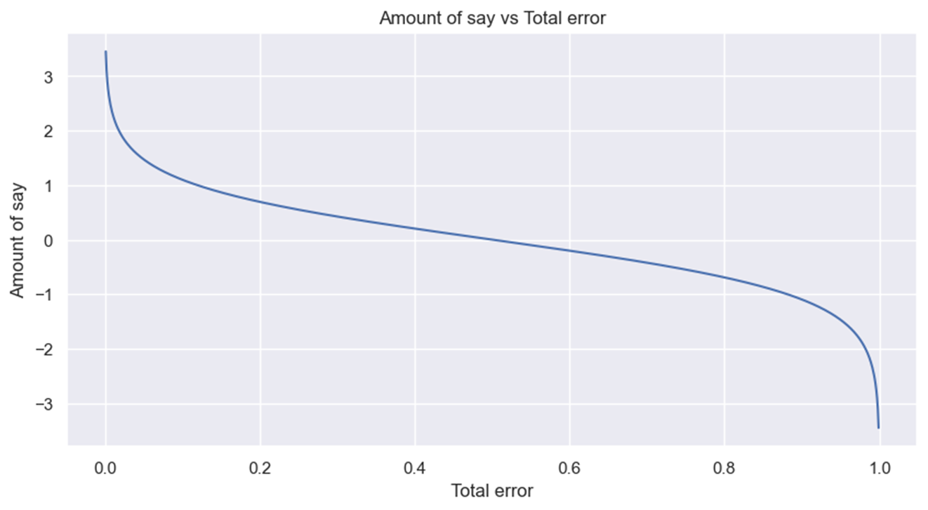
If the total error is close to 0, the amount of say is a big positive number, indicating the stump gives many contributions to the final prediction. On the other hand, if the total error is close to 1, the amount of say is a big negative number, giving much penalty for the misclassification the stump produces. If the total error is 0.5, the stump doesn’t do anything for the final prediction.
Step 3. Update sample weight
AdaBoost will increase the weights of incorrectly labeled observations and decrease the weights of correctly labeled observations. The new sample weight influences the next Decision Stump: observations with larger weights are paid more attention to.
To update the sample weight, use the formula
- For incorrectly labeled observations:

- For correctly labeled observations:

You need to normalize the new sample weights such that their sum equals 1 before continuing to the next step, using the formula

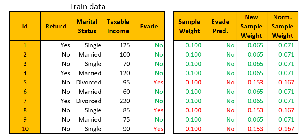
These calculations are summarized in the table below. The green observations are correctly labeled and the red ones are incorrectly labeled by the current stump.
Step 4. Repeat
A new Decision Stump is created using the weighted impurity function, i.e. weighted Gini Index, where normalized sample weight is considered in determining the proportion of observations per class. Alternatively, another way to create a Decision Stump is to use bootstrapped data based on normalized sample weight.
Since normalized sample weight has a sum of 1, it can be considered as a probability that a particular observation is picked when bootstrapping. So, observations with Ids 5, 8, and 10 are more probable to be picked and hence the Decision Stump is more focused on them.
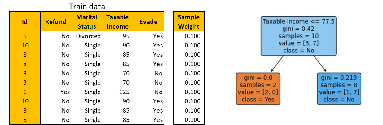
The bootstrapped data is shown below. Note that you may get different bootstrapped data due to randomness. Build a Decision Stump as before.
You see that there’s one misclassified observation. So, the amount of say is 1.099. Update the sample weight and normalize with respect to the sum of weights of only bootstrapped observations. These calculations are summarized in the table below.

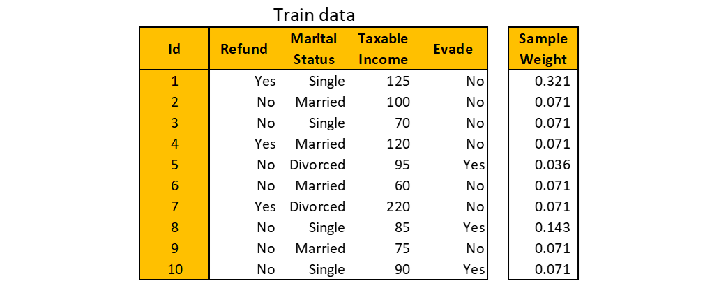
The bootstrapped observations go back to the pool of train data and the new sample weight becomes as shown below. You can then bootstrap the train data again using the new sample weight for the third Decision Stump and the process goes on.
Prediction
Let’s say you iterate the steps six times. Thus, you have six Decision Stumps. To make predictions, traverse each stump using the test data and group the predicted classes. The group with the largest amount of say represents the final prediction of AdaBoost.
To illustrate, the first two Decision Stumps you built have the amount of say 0.424 and 1.099, respectively. Both stumps predict Evade = No since for the taxable income, 77.5 < 80 ≤ 97.5 (80 is the value of Taxable Income for the test observation). Let’s say the other four Decision Stumps predict and have the following amount of say.
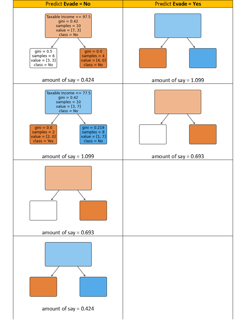
Since the sum of the amount of say of all stumps that predict Evade = No is 2.639, bigger than the sum of the amount of say of all stumps that predict Evade = Yes (which is 1.792), then the final AdaBoost prediction is Evade = No.
Since both are boosting methods, AdaBoost and Gradient Boosting have a similar workflow. There are two main differences though:
- Gradient Boosting uses trees larger than a Decision Stump. In this story, we limit the trees to have a maximum of 3 leaf nodes, which is a hyperparameter that can be changed at will.
- Instead of using sample weight to guide the next Decision Stump, Gradient Boosting uses the residual made by the Decision Tree to guide the next tree.
Recall the tax evasion dataset. You will use Gradient Boosting to predict whether a person will comply to pay taxes based on three features: Taxable Income, Marital Status, and Refund.
Step 1. Initialize a root
A root is a Decision Tree with zero depth. It doesn’t consider any feature to do prediction: it uses Evade itself to predict on Evade. How does it do this? Encode Evade using the mapping No → 0 and Yes → 1. Then, take the average, which is 0.3. This is called the prediction probability (the value is always between 0 and 1) and is denoted by p.
Since 0.3 is less than the threshold of 0.5, the root will predict No for every train observation. In other words, the prediction is always the mode of Evade. Of course, this is a very bad initial prediction. To improve the performance, you can calculate the log(odds) to be used in the next step using the formula

Step 2. Calculate the residual to fit a Decision Tree into
To simplify notations, let the encoded column of Evade be denoted by y. Residual is defined simply by r = y − p, where p is the prediction probability calculated from the latest log(odds) using its inverse function

Build a Decision Tree to predict the residual using all train observations. Note that this is a regression task.
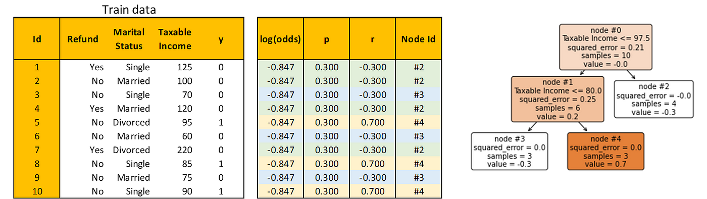
Step 3. Update log(odds)
Note that I also added a Node Id column that explains the index of the node in the Decision Tree where each observation is predicted. In the table above, each observation is color-coded to easily see which observation goes to which node.
To combine the predictions of the initial root and the Decision Tree you just built, you need to transform the predicted values in the Decision Tree such that they match the log(odds) in the initial root.
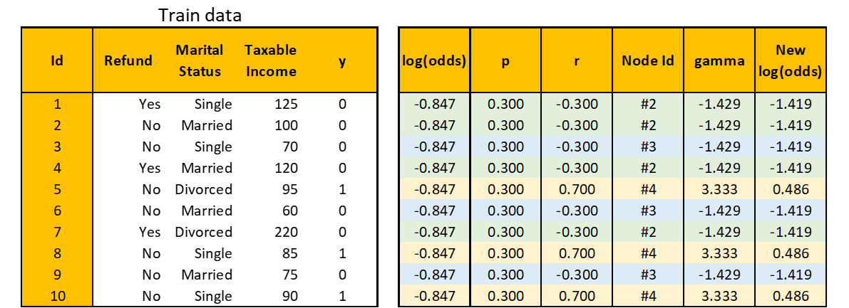
For example, let dᵢ denote the set of observation Ids in node #i, i.e. d₂ = {1, 2, 4, 7}. Then the transformation for node #2 is

Do the same calculation to node #3 and node #4, you get γ for all training observations as the following table. Now you can update the log(odds) using the formula

where α is the learning rate of Gradient Boosting and is a hyperparameter. Let’s set α = 0.4, then the complete calculation of updating log(odds) can be seen below.
Step 4. Repeat
Using the new log(odds), repeat Step 2 and Step 3. Here’s the new residual and the Decision Tree built to predict it.
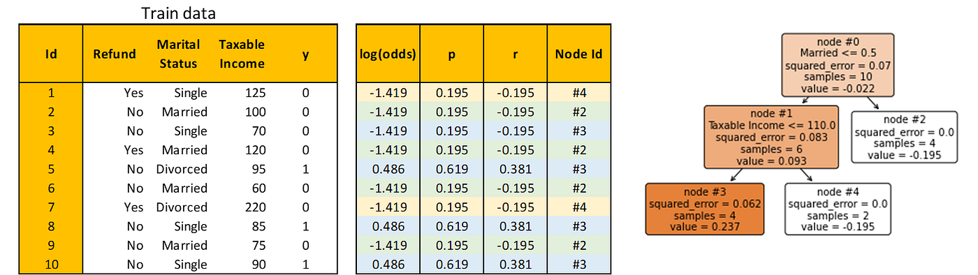
Calculate γ as before. For example, consider node #3, then

Using γ, calculate the new log(odds) as before. Here’s the complete calculation

You can repeat the process as many times as you like. For this story, however, to avoid things getting out of hand, we will stop the iteration now.
Prediction
To do prediction on test data, first, traverse each Decision Tree until reaching a leaf node. Then, add the log(odds) of the initial root with all the γ of the corresponding leaf nodes scaled by the learning rate.
In our example, the test observation lands on node #3 of both Decision Trees. Hence, the summation becomes -0.847 + 0.4 × (-1.429 + 1.096) = -0.980. Convert to prediction probability

Since 0.273 < 0.5, predict Evade = No.
You’ve learned in great detail Random Forest, AdaBoost, and Gradient Boosting, and applied them to a simple dummy dataset. Now, not only you can build them using established libraries, but you also confidently know how they work from the inside out, the best practices to use them, and how to improve their performance.
Congrats!
🔥 Thanks! If you enjoy this story and want to support me as a writer, consider becoming a member. For only $5 a month, you’ll get unlimited access to all stories on Medium. If you sign up using my link, I’ll earn a small commission.
🔖 Want to know more about how gradient descent and many other optimizers work? Continue reading:
Optimization Methods from Scratch
My Best Stories
Random Forest is one of the most popular bagging methods. What’s bagging you ask? It’s an abbreviation for bootstrapping + aggregating. The goal of bagging is to reduce the variance of a single estimator, i.e. the variance of a single Decision Tree in the case of Random Forest.
To be concrete, let’s use a dummy dataset throughout this story. Suppose you have the following tax evasion dataset. Your task is to predict whether a person will comply to pay taxes (the Evade column) based on features like Taxable Income (in thousand dollars), Marital Status, and whether a Refund is implemented or not.
Random Forest consists of these three steps:
Step 1. Create a bootstrapped data
Given an original train data with m observations and n features, sample m observations randomly with repetition. The keyword here is “with repetition”. This means it’s most likely that some observations are picked more than once.
Below is an example of bootstrapped data from the original train data above. You might have different bootstrapped data due to randomness.
Step 2. Build a Decision Tree
The decision tree is built:
- using the bootstrapped data, and
- considering a random subset of features at each node (the number of features considered is usually the square root of n).
Step 3. Repeat
Step 1 and Step 2 are iterated many times. For example, using the tax evasion dataset with six iterations, you’ll get the following Random Forest.
Note that Random Forest is not deterministic since there’s a random selection of observations and features at play. These random selections are why Random Forest reduces the variance of a Decision Tree.
Predict, aggregate, and evaluate
To make predictions using Random Forest, traverse each Decision Tree using the test data. For our example, there’s only one test observation on which six Decision Trees respectively give predictions No, No, No, Yes, Yes, and No for the “Evade” target. Do majority voting from these six predictions to make a single Random Forest prediction: No.
Combining predictions of Decision Trees into a single prediction of Random Forest is called aggregating. While majority voting is used for classification problems, the aggregating method for regression problems uses the mean or median of all Decision Tree predictions as a single Random Forest prediction.
The creation of bootstrapped data allows some train observations to be unseen by a subset of Decision Trees. These observations are called out-of-bag samples and are useful for evaluating the performance of Random Forest. To obtain validation accuracy (or any metric of your choice) of Random Forest:
- run out-of-bag samples through all Decision Trees that were built without them,
- aggregate the predictions, and
- compare the aggregated predictions with the true labels.
Unlike Random Forest, AdaBoost (Adaptive Boosting) is a boosting ensemble method where simple Decision Trees are built sequentially. How simple? The trees consist of only a root and two leaves, so simple that they have their own name: Decision Stumps. Here are two main differences between Random Forest and AdaBoost:
- Decision Trees in Random Forest have equal contributions to the final prediction, whereas Decision Stumps in AdaBoost have different contributions, i.e. some stumps have more say than others.
- Decision Trees in Random Forest are built independently, whereas each Decision Stump in AdaBoost is made by taking the previous stump’s mistake into account.
Decision Stumps are too simple; they are slightly better than random guessing and have a high bias. The goal of boosting is to reduce the bias of a single estimator, i.e. the bias of a single Decision Stump in the case of AdaBoost.
Recall the tax evasion dataset. You will use AdaBoost to predict whether a person will comply to pay taxes based on three features: Taxable Income, Marital Status, and Refund.
Step 1. Initialize sample weight and build a Decision Stump
Remember that a Decision Stump in AdaBoost is made by taking the previous stump’s mistake into account. To do that, AdaBoost assigns a sample weight to each train observation. Bigger weights are assigned to misclassified observations by the current stump, informing the next stump to pay more attention to those misclassified observations.
Initially, since there are no predictions made yet, all observations are given the same weight of 1/m. Then, a Decision Stump is built just like creating a Decision Tree with depth 1.
Step 2. Calculate the amount of say for the Decision Stump
This Decision Stump yields 3 misclassified observations. Since all observations have the same sample weight, the total error in terms of sample weight is 1/10 + 1/10 + 1/10 = 0.3.
The amount of say can then be calculated using the formula
To understand why the formula makes sense, let’s plot the amount of say vs total error. Note that total error is only defined on the interval [0, 1].
If the total error is close to 0, the amount of say is a big positive number, indicating the stump gives many contributions to the final prediction. On the other hand, if the total error is close to 1, the amount of say is a big negative number, giving much penalty for the misclassification the stump produces. If the total error is 0.5, the stump doesn’t do anything for the final prediction.
Step 3. Update sample weight
AdaBoost will increase the weights of incorrectly labeled observations and decrease the weights of correctly labeled observations. The new sample weight influences the next Decision Stump: observations with larger weights are paid more attention to.
To update the sample weight, use the formula
- For incorrectly labeled observations:
- For correctly labeled observations:
You need to normalize the new sample weights such that their sum equals 1 before continuing to the next step, using the formula
These calculations are summarized in the table below. The green observations are correctly labeled and the red ones are incorrectly labeled by the current stump.
Step 4. Repeat
A new Decision Stump is created using the weighted impurity function, i.e. weighted Gini Index, where normalized sample weight is considered in determining the proportion of observations per class. Alternatively, another way to create a Decision Stump is to use bootstrapped data based on normalized sample weight.
Since normalized sample weight has a sum of 1, it can be considered as a probability that a particular observation is picked when bootstrapping. So, observations with Ids 5, 8, and 10 are more probable to be picked and hence the Decision Stump is more focused on them.
The bootstrapped data is shown below. Note that you may get different bootstrapped data due to randomness. Build a Decision Stump as before.
You see that there’s one misclassified observation. So, the amount of say is 1.099. Update the sample weight and normalize with respect to the sum of weights of only bootstrapped observations. These calculations are summarized in the table below.
The bootstrapped observations go back to the pool of train data and the new sample weight becomes as shown below. You can then bootstrap the train data again using the new sample weight for the third Decision Stump and the process goes on.
Prediction
Let’s say you iterate the steps six times. Thus, you have six Decision Stumps. To make predictions, traverse each stump using the test data and group the predicted classes. The group with the largest amount of say represents the final prediction of AdaBoost.
To illustrate, the first two Decision Stumps you built have the amount of say 0.424 and 1.099, respectively. Both stumps predict Evade = No since for the taxable income, 77.5 < 80 ≤ 97.5 (80 is the value of Taxable Income for the test observation). Let’s say the other four Decision Stumps predict and have the following amount of say.
Since the sum of the amount of say of all stumps that predict Evade = No is 2.639, bigger than the sum of the amount of say of all stumps that predict Evade = Yes (which is 1.792), then the final AdaBoost prediction is Evade = No.
Since both are boosting methods, AdaBoost and Gradient Boosting have a similar workflow. There are two main differences though:
- Gradient Boosting uses trees larger than a Decision Stump. In this story, we limit the trees to have a maximum of 3 leaf nodes, which is a hyperparameter that can be changed at will.
- Instead of using sample weight to guide the next Decision Stump, Gradient Boosting uses the residual made by the Decision Tree to guide the next tree.
Recall the tax evasion dataset. You will use Gradient Boosting to predict whether a person will comply to pay taxes based on three features: Taxable Income, Marital Status, and Refund.
Step 1. Initialize a root
A root is a Decision Tree with zero depth. It doesn’t consider any feature to do prediction: it uses Evade itself to predict on Evade. How does it do this? Encode Evade using the mapping No → 0 and Yes → 1. Then, take the average, which is 0.3. This is called the prediction probability (the value is always between 0 and 1) and is denoted by p.
Since 0.3 is less than the threshold of 0.5, the root will predict No for every train observation. In other words, the prediction is always the mode of Evade. Of course, this is a very bad initial prediction. To improve the performance, you can calculate the log(odds) to be used in the next step using the formula
Step 2. Calculate the residual to fit a Decision Tree into
To simplify notations, let the encoded column of Evade be denoted by y. Residual is defined simply by r = y − p, where p is the prediction probability calculated from the latest log(odds) using its inverse function
Build a Decision Tree to predict the residual using all train observations. Note that this is a regression task.
Step 3. Update log(odds)
Note that I also added a Node Id column that explains the index of the node in the Decision Tree where each observation is predicted. In the table above, each observation is color-coded to easily see which observation goes to which node.
To combine the predictions of the initial root and the Decision Tree you just built, you need to transform the predicted values in the Decision Tree such that they match the log(odds) in the initial root.
For example, let dᵢ denote the set of observation Ids in node #i, i.e. d₂ = {1, 2, 4, 7}. Then the transformation for node #2 is
Do the same calculation to node #3 and node #4, you get γ for all training observations as the following table. Now you can update the log(odds) using the formula
where α is the learning rate of Gradient Boosting and is a hyperparameter. Let’s set α = 0.4, then the complete calculation of updating log(odds) can be seen below.
Step 4. Repeat
Using the new log(odds), repeat Step 2 and Step 3. Here’s the new residual and the Decision Tree built to predict it.
Calculate γ as before. For example, consider node #3, then
Using γ, calculate the new log(odds) as before. Here’s the complete calculation
You can repeat the process as many times as you like. For this story, however, to avoid things getting out of hand, we will stop the iteration now.
Prediction
To do prediction on test data, first, traverse each Decision Tree until reaching a leaf node. Then, add the log(odds) of the initial root with all the γ of the corresponding leaf nodes scaled by the learning rate.
In our example, the test observation lands on node #3 of both Decision Trees. Hence, the summation becomes -0.847 + 0.4 × (-1.429 + 1.096) = -0.980. Convert to prediction probability
Since 0.273 < 0.5, predict Evade = No.
You’ve learned in great detail Random Forest, AdaBoost, and Gradient Boosting, and applied them to a simple dummy dataset. Now, not only you can build them using established libraries, but you also confidently know how they work from the inside out, the best practices to use them, and how to improve their performance.
Congrats!
🔥 Thanks! If you enjoy this story and want to support me as a writer, consider becoming a member. For only $5 a month, you’ll get unlimited access to all stories on Medium. If you sign up using my link, I’ll earn a small commission.
🔖 Want to know more about how gradient descent and many other optimizers work? Continue reading:
Optimization Methods from Scratch
My Best Stories
Denial of responsibility! Techno Blender is an automatic aggregator of the all world’s media. In each content, the hyperlink to the primary source is specified. All trademarks belong to their rightful owners, all materials to their authors. If you are the owner of the content and do not want us to publish your materials, please contact us by email – [email protected]. The content will be deleted within 24 hours.