
Understanding Partial Effects, Main Effects, and Interaction Effects in a Regression Model | by Sachin Date | Jul, 2022
We’ll learn how to identify and measure these effects in a regression model using suitable examples.
In this article, we’ll figure out how to calculate the partial (or marginal) effect, the main effect, and the interaction effect of regression variables on the response variable of a regression model. We’ll also learn how to interpret the coefficients of the regression model in terms of the appropriate effect.
Let’s begin with the partial effect, also known as the marginal effect.
In a regression model, the partial effect of a regression variable is the change in the value of the response variable for every unit change in the regression variable.
In the language of Calculus, the partial effect is the partial derivative of the expected value of the response w.r.t. the regression variable of interest.
Let’s see three increasingly complex examples of the partial effect.
Consider the following linear regression model:

In the above model, y is the dependent variable, and x_1, x_2 are regression variables. y_i, x_i_1 and x_i_2 are the values corresponding to the the ith observation, i.e., the ith row of the data set.
β_0 is the intercept. ϵ_i is the error term that captures the variance in y_i that the model has not been able to explain.
When we fit the above model on a data set, we are estimating the expected, i.e. the mean, value of y_i for some observed values of x_i_1 and x_i_2. If we apply the Expectation operator E(.) to both sides of equation (1), we get the following equation. Notice that the error term has disappeared since its expected value is zero:

The partial effects of x_i_1 and x_i_2 (or in general, x_1 and x_2) on the expected value of y_i are the respective partial derivatives of y_i w.r.t. x_i_1 and x_i_2, as follows:

In case of a linear model containing only linear terms, the partial effects are simply the respective coefficients. In such a model, the partial effects are constants.
Now, let’s make this model a bit complex by adding a quadratic term and an interaction term:

This model is still a linear model since its linear in its coefficients. However, the partial effect of x_i_2 on the expected value of y_i is no longer constant. Instead, the effect depends on the current values of x_i_2 and x_i_1 as follows:

Finally, let’s look at the following nonlinear model containing the exponentiated mean function. This model is used for modeling the mean function of a Poisson process:

In this model, the partial effect of x_i_1 is as follows:

We see that in this case, the change in the expected value of y_i per unit change in x_i_1 is not only not constant, but it depends on current value of every single variable and the value of all coefficients.
Let’s now turn our attention to what the main effect means in a regression model.
In a linear regression model containing only linear terms, the main effect of each regression variable is the same as the partial effect of that variable.
Thus, in the following model that we saw earlier:
The main effects in the above model are simply β_1 and β_2.
Since this model contains only linear terms, it is sometimes called the main effects model.
The interpretation of main effects becomes interesting when the model contains quadratic, interaction, nonlinear or loglinear terms.
In models of the following kind:
The coefficients β_1 and β_2 associated with variables x_1 and x_2 can no longer be interpreted as the main effects associated with these variables. So how are main effects calculated in such models?
One way to do so is to calculate the partial effect of each variable and compute it for each row of the data set. Then take the mean of all such partial effects.
For instance, in the above model, the partial effect of x_i_1 (or in general x_1) on E(y_i) is calculated as follows:

To calculate the main effect of x_i_1, we must calculate the above partial effect for each row in the data set and take the average of all those partial effects:

While the above formula provides a sound means to calculate the main effect, it is an approximation that is applicable really only to the data set in hand. In fact, it is debatable whether the main effect should be calculated in such models, or it should be simply ignored in case of such models that do not contain only linear terms.
Finally, let’s review what is meant by interaction effect.
Let’s extend our linear model by including an additional term as follows:

The term x_i_1*x_i_2 which is the multiplication of the observed values of the two regression variables represents the interaction between the two variables. This time, when we take the partial derivative of the expected value of y_i w.r.t. x_i_1, we get the following:

The change in E(y_i) with respect to x_i_1 is no longer just β_1. Due to the presence of the interaction term, it is β_1 plus a quantity that depends on the current value of x_i_2 times the coefficient β_3 of the interaction term. If the coefficient β_3 happens to be negative, it will reduce the net change in y_i for each unit change in x_i_1, and if β_4 is positive, it will boost it (assuming x_i_2 is positive in both cases).
If we take a second derivative of E(y_i), this time w.r.t. x_i_2, we get the following:

We can now see what the effect of the interaction term (x_i_1*x_i_2) is on the model.
The coefficient β_3 measures the amount by which the rate of change of E(y_i) w.r.t. x_i_1 changes for each unit change in x_i_2. Thus, β_3 measures the degree of the interaction between x_i_1 and x_i_2.
β_3 is called the interaction effect.
Interpretation of the interaction term’s coefficient
Just as with the main effect, the coefficient of the interaction term can be interpreted to be the size of the interaction effect, but only in a linear model that contains only linear terms and an interaction term.
For all other cases, and especially in nonlinear models, the coefficient of the interaction term caries no significance in it’s ability to indicate the size of the interaction term. To illustrate, consider the following nonlinear model which estimates the mean as an exponentiated linear combination of regression variables. This model is commonly used to represent the non-negative Poisson process mean in a Poisson regression model:
A first derivative of E(y_i) w.r.t. x_i_1 yields the following partial effect of x_i_1 on E(y_i):

Clearly, as against a linear model with only linear terms, in the above partial effect, the coefficient β_3 of x_i_1 no longer provides us any clues to the size of the main effect of x_i_1.
A second derivative of E(y_i), this time w.r.t. x_i_2 delivers an even messier situation:

The key takeaway is that in a nonlinear model, one should not try to ascribe any meaning to the coefficient of the interaction effect.
The benefits of adding interaction effects
One may wonder why one would want to introduce interaction terms in a regression model.
Interaction terms are a useful device for representing the effect of one regression variable on another one within the same model. The main effect measures how sensitive the response variable is to changes in the values of a single regressor, keeping the values of all other variables constant (or at their respective mean values). The interaction effect measures how sensitive is this sensitivity of E(y) w.r.t. x, to changes in another variable z especially when z also happens to interact with x.
Here are a couple of examples that illustrate the use of the interaction effect:
- In a model that studies the relationship of a person’s income with characteristics such as age, sex and education, one may want to know by what amount does the income change for each unit change in education level, if the person happens to be a female versus a male. In other words, are females participants in the study seen to have benefited from additional educational any more (or any less) than male participants, all other things staying the same. If we represent the relationships using a linear model of income regressed on age, sex, education and sex*education, the interaction effect is the coefficient of sex*education.
- In a model that studies the impact of temperature and particulate air population on rainfall intensity, the main effects will measure by how the rainfall amount changes for unit changes in temperature or air pollution respectively, while the interaction effect could measure by what amount will the change in rainfall w.r.t. a unit change in pollution level, will itself change for each unit change in temperature.
In the rest of the article, we’ll build a model containing an interaction effect. Specifically, we will estimate academic performance of students in two Portuguese schools by regressing their performance on a set of six variables and one interaction term. The complete data set can be downloaded from UC Irvine’s machine learning repository website. A curated subset of the data set in which we have dropped most of the columns from the original data set, and coded all binary variables as 0 or 1, is available for download from here.
Here’s how a portion of this curated data set looks like:

Each row contains the test performance of a unique student. The dependent variable (G1) is their first period grade in Math and it varies from 0 through 20. We will regress grade on a number of factors and one interaction term as follows:

Here, failures is the number of times the student failed in past classes. The value goes from 0 through 4. It is right-censored at 4.
schoolsup and famsup are boolean variables indicating whether the student received any extra educational support from their school or from their family respectively. A value of 1 indicates they received some support, and 0 indicates they received no support.
studytime contains the amount of time the student spent studying per week. Its value is intervalized to go from 1 through 4 in increments of 1, where 1 means < 2 hours, 2 means 2 to 5 hours, 3 means 5 to 10 hours and 4 means greater than 10 hours.
goout represents the extent to which the student hangs out with friends outside the house. Its an integer value ranging from 1 through 5 where 1 means very low extent, and 5 means very high extent.
sex is a boolean variable (1=Female and 0=Male).
We have also included an interaction term in this model called (failures*sex).
If we differentiate G1 w.r.t. sex, we get the following partial effect of sex on G1:
This equation gives us the difference between the average grade of male and female students. Due to the presence of the interaction term, this difference is also dependent on the number of past failures.
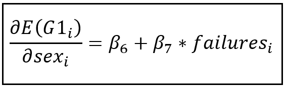
If we differentiate one more time, this time w.r.t. failures, we get the following:

β_7 is the rate at which the difference between the average grade of male and female students changes for each unit change in number of past failures.
Thus β_7 estimates the interaction effect between sex and number of failures.
Let’s build and train this model on the data set. We’ll use Python and the Pandas data analysis library and the statsmodels statistical models library.
Let’s start by importing all the required packages.
import pandas as pd
from patsy import dmatrices
import statsmodels.api as sm
Next, we’ll use Pandas to load the data set into a Pandas DataFrame:
df = pd.read_csv('uciml_portuguese_students_math_performance_subset.csv', header=0)
We’ll now form the regression expression in Patsy syntax. We do not need to explicitly specify the intercept. Patsy will automatically add it to the X matrix in a following step.
reg_exp = 'G1 ~ failures + schoolsup + famsup + studytime + goout + sex + I(failures*sex)'
Let’s carve out the X and y matrices:
y_train, X_train = dmatrices(reg_exp, df, return_type='dataframe')
Here is how the carved out design matrices look like:


Notice that Patsy has added a placeholder column in X for the intercept β_0, and it has also added the column containing the interaction term failures*sex.
We’ll now build and train the model on (y_train, X_train):
olsr_model = sm.OLS(endog=y_train, exog=X_train)olsr_model_results = olsr_model.fit()
Let’s also print the training summary:
print(olsr_model_results.summary())
We see the following output (I have highlighted a few interesting elements):

How to interpret the regression model’s training performance
The adjusted R-squared is 0.210 implying that the model has been able to explain 21% of the variance in the G1 score. The F-statistic of the F-test is 15.96 and it is significant at a p value of < .001, meaning that the model’s variables are jointly highly significant. The model is able to do a much better job of explaining the variance in student performance than a simple mean model.
Next, let’s note that almost all coefficients are statistically significant at a p value of < .05 or lower. famsup is significant at a p of .061 and the interaction term failures*sex is significant at a p of .073.
The equation of the fitted model is as follows:

Interpretation of coefficients
Let’s see how to interpret the various coefficients of the fitted model.
The partial effect of failures on G1 is given by the following equation:

The coefficient of failures is -1.7986. Due to the presence of the interaction term (failures*sex) , -1.7986 is no longer the main effect of past failures on the expected G1 score. In fact, one should not ascribe any meaning to the value of this coefficient except in the situation where the coefficient of sex is 0, which it isn’t in this case. The best we can do is to calculate the partial effect of failures on E(G1) for each row in the data set and consider the average of all those values as the main effect of failures on E(G1). As mentioned earlier, this strategy is of dubious value and a safer approach would be to altogether abandon the pursuit of computing the main effect of failures, given the presence of the interaction term.
Exactly same set of considerations hold while interpreting the coefficient of sex in the training output.
The considerations change dramatically while interpreting the coefficients of schoolsup, famsup, studytime and goout. None of these variables are involved in the interaction term (failures*sex) leading to a straightforward interpretation of their coefficients as follows.
Across all students, the estimated mean reduction in their G1 score for each unit increase in the amount of time they spend in “going out” (goout) is .3105. This is partial effect of goout on E(G1). It is also the main effect of goout on E(G1).
Similarly, the coefficients of the boolean variables schoolsup and famsup are the respective partial effects of that variable on E(G1), and they are also the respective main effect of that variable on E(G1). Surprisingly, both coefficients are negative, indicating that students who received additional support from their school or their family did on average worse than those who did not receive support. One way to explain this result is to theorize that most of the students who are receiving additional support are receiving them because they are faring poorly in their math grades.
On the other hand, studytime has an unsurprisingly positive relationship with the G1 score with each unit increase in studytime leading to an increase in the G1 score by 0.5848.
Lastly, let’s examine the interaction effect of failures with sex. The coefficient of the interaction term (failures*sex) is positive indicating that for each unit increase in number of past failures experienced by the student, the edge that male students seem to have over female students in the G1 score rapidly evaporates, reducing as it does by 0.7312 points. This conclusion is borne out by taking the derivative of E(G1) w.r.t. sex which gives us the partial effect of sex on the mean G1 score:

From the equation, we can see that the partial effect reverse sign very quickly with increase in number of past failures:

The following table and graph shows another view (an empirical view) into the same situation. It shows the mean scores of female and male students calculated from the data set, for each value of past failures:
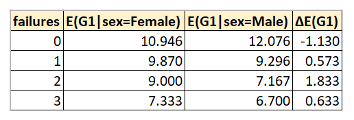
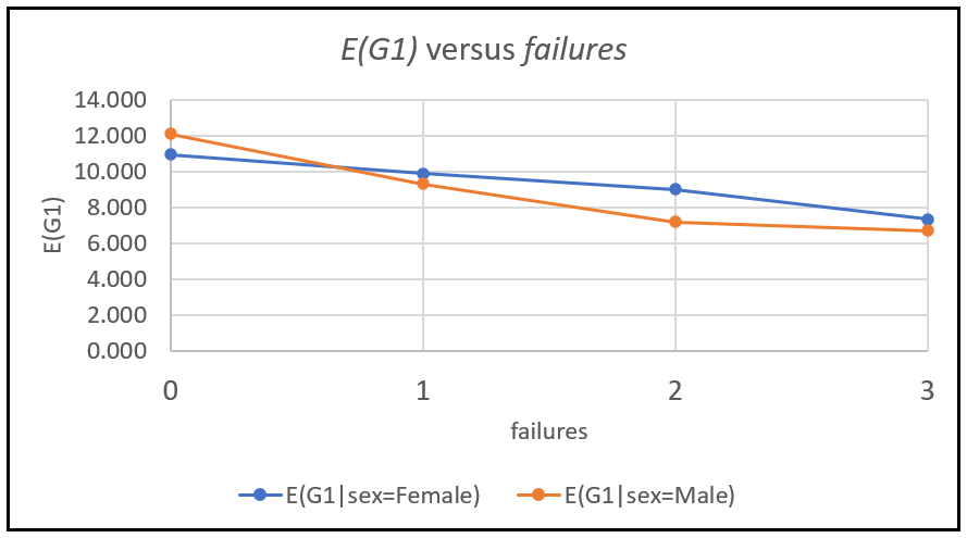
As expected, we see the empirical outcome agrees with the modeled outcome i.e. the one using the equation for the partial effect of sex of E(G1). The difference between male and female students’ G1 score quickly reverses with increase in number of past failures. Higher levels of past failures seem to adversely affecting male students’ scores much more than they do female students’ scores. The reasons behind this effect may well be rooted in some of the other factors in the model, or they may be unobserved effects that have leaked into the error term of the model.
Observations of this kind are possible via the inclusion of interaction terms. We would not have been able to easily spot this pattern by including only the main effects for sex and failures in the regression model.
- In a regression model, the partial effect or marginal effect of a regression variable is the change in the value of the response variable for every unit change in the regression variable.
- In a linear model that contains only linear terms, i.e. no quadratic, log, and other kinds of nonlinear terms, the main effect of each regression variable is the same as its partial effect.
- For all other models, the main effect of variable can be calculated by averaging the partial effect of the variable over the entire data set. This is at best an approximation that is applicable essentially only to the data set in hand. And therefore, some practitioners prefer to altogether ignore the main effects in such kinds of models.
- Interaction terms help the modeler estimate the effect of one regression variable on other variables in the model in their joint ability to explain the variance in the response variable.
- In certain simple linear models, the coefficient of the interaction term can be used to estimate the size of the interaction effect. However, in most models, one should not ascribe any meaning to the coefficient of the interaction term.
Data set
Data set of student performance sourced from UCI Machine Learning Repository under their citation policy.
Dua, D. and Graff, C. (2019). UCI Machine Learning Repository [http://archive.ics.uci.edu/ml]. Irvine, CA: University of California, School of Information and Computer Science.
The curated version of the data set used in this article is available for download from here.
Paper
P. Cortez and A. Silva. Using Data Mining to Predict Secondary School Student Performance. In A. Brito and J. Teixeira Eds., Proceedings of 5th FUture BUsiness TEChnology Conference (FUBUTEC 2008) pp. 5–12, Porto, Portugal, April, 2008, EUROSIS, ISBN 978–9077381–39–7.
[Web Link]
Images
All images in this article are copyright Sachin Date under CC-BY-NC-SA, unless a different source and copyright are mentioned underneath the image.
If you liked this article, please follow me at Sachin Date to receive tips, how-tos and programming advice on topics devoted to regression, time series analysis, and forecasting.

We’ll learn how to identify and measure these effects in a regression model using suitable examples.
In this article, we’ll figure out how to calculate the partial (or marginal) effect, the main effect, and the interaction effect of regression variables on the response variable of a regression model. We’ll also learn how to interpret the coefficients of the regression model in terms of the appropriate effect.
Let’s begin with the partial effect, also known as the marginal effect.
In a regression model, the partial effect of a regression variable is the change in the value of the response variable for every unit change in the regression variable.
In the language of Calculus, the partial effect is the partial derivative of the expected value of the response w.r.t. the regression variable of interest.
Let’s see three increasingly complex examples of the partial effect.
Consider the following linear regression model:
In the above model, y is the dependent variable, and x_1, x_2 are regression variables. y_i, x_i_1 and x_i_2 are the values corresponding to the the ith observation, i.e., the ith row of the data set.
β_0 is the intercept. ϵ_i is the error term that captures the variance in y_i that the model has not been able to explain.
When we fit the above model on a data set, we are estimating the expected, i.e. the mean, value of y_i for some observed values of x_i_1 and x_i_2. If we apply the Expectation operator E(.) to both sides of equation (1), we get the following equation. Notice that the error term has disappeared since its expected value is zero:
The partial effects of x_i_1 and x_i_2 (or in general, x_1 and x_2) on the expected value of y_i are the respective partial derivatives of y_i w.r.t. x_i_1 and x_i_2, as follows:
In case of a linear model containing only linear terms, the partial effects are simply the respective coefficients. In such a model, the partial effects are constants.
Now, let’s make this model a bit complex by adding a quadratic term and an interaction term:
This model is still a linear model since its linear in its coefficients. However, the partial effect of x_i_2 on the expected value of y_i is no longer constant. Instead, the effect depends on the current values of x_i_2 and x_i_1 as follows:
Finally, let’s look at the following nonlinear model containing the exponentiated mean function. This model is used for modeling the mean function of a Poisson process:
In this model, the partial effect of x_i_1 is as follows:
We see that in this case, the change in the expected value of y_i per unit change in x_i_1 is not only not constant, but it depends on current value of every single variable and the value of all coefficients.
Let’s now turn our attention to what the main effect means in a regression model.
In a linear regression model containing only linear terms, the main effect of each regression variable is the same as the partial effect of that variable.
Thus, in the following model that we saw earlier:
The main effects in the above model are simply β_1 and β_2.
Since this model contains only linear terms, it is sometimes called the main effects model.
The interpretation of main effects becomes interesting when the model contains quadratic, interaction, nonlinear or loglinear terms.
In models of the following kind:
The coefficients β_1 and β_2 associated with variables x_1 and x_2 can no longer be interpreted as the main effects associated with these variables. So how are main effects calculated in such models?
One way to do so is to calculate the partial effect of each variable and compute it for each row of the data set. Then take the mean of all such partial effects.
For instance, in the above model, the partial effect of x_i_1 (or in general x_1) on E(y_i) is calculated as follows:
To calculate the main effect of x_i_1, we must calculate the above partial effect for each row in the data set and take the average of all those partial effects:
While the above formula provides a sound means to calculate the main effect, it is an approximation that is applicable really only to the data set in hand. In fact, it is debatable whether the main effect should be calculated in such models, or it should be simply ignored in case of such models that do not contain only linear terms.
Finally, let’s review what is meant by interaction effect.
Let’s extend our linear model by including an additional term as follows:
The term x_i_1*x_i_2 which is the multiplication of the observed values of the two regression variables represents the interaction between the two variables. This time, when we take the partial derivative of the expected value of y_i w.r.t. x_i_1, we get the following:
The change in E(y_i) with respect to x_i_1 is no longer just β_1. Due to the presence of the interaction term, it is β_1 plus a quantity that depends on the current value of x_i_2 times the coefficient β_3 of the interaction term. If the coefficient β_3 happens to be negative, it will reduce the net change in y_i for each unit change in x_i_1, and if β_4 is positive, it will boost it (assuming x_i_2 is positive in both cases).
If we take a second derivative of E(y_i), this time w.r.t. x_i_2, we get the following:
We can now see what the effect of the interaction term (x_i_1*x_i_2) is on the model.
The coefficient β_3 measures the amount by which the rate of change of E(y_i) w.r.t. x_i_1 changes for each unit change in x_i_2. Thus, β_3 measures the degree of the interaction between x_i_1 and x_i_2.
β_3 is called the interaction effect.
Interpretation of the interaction term’s coefficient
Just as with the main effect, the coefficient of the interaction term can be interpreted to be the size of the interaction effect, but only in a linear model that contains only linear terms and an interaction term.
For all other cases, and especially in nonlinear models, the coefficient of the interaction term caries no significance in it’s ability to indicate the size of the interaction term. To illustrate, consider the following nonlinear model which estimates the mean as an exponentiated linear combination of regression variables. This model is commonly used to represent the non-negative Poisson process mean in a Poisson regression model:
A first derivative of E(y_i) w.r.t. x_i_1 yields the following partial effect of x_i_1 on E(y_i):
Clearly, as against a linear model with only linear terms, in the above partial effect, the coefficient β_3 of x_i_1 no longer provides us any clues to the size of the main effect of x_i_1.
A second derivative of E(y_i), this time w.r.t. x_i_2 delivers an even messier situation:
The key takeaway is that in a nonlinear model, one should not try to ascribe any meaning to the coefficient of the interaction effect.
The benefits of adding interaction effects
One may wonder why one would want to introduce interaction terms in a regression model.
Interaction terms are a useful device for representing the effect of one regression variable on another one within the same model. The main effect measures how sensitive the response variable is to changes in the values of a single regressor, keeping the values of all other variables constant (or at their respective mean values). The interaction effect measures how sensitive is this sensitivity of E(y) w.r.t. x, to changes in another variable z especially when z also happens to interact with x.
Here are a couple of examples that illustrate the use of the interaction effect:
- In a model that studies the relationship of a person’s income with characteristics such as age, sex and education, one may want to know by what amount does the income change for each unit change in education level, if the person happens to be a female versus a male. In other words, are females participants in the study seen to have benefited from additional educational any more (or any less) than male participants, all other things staying the same. If we represent the relationships using a linear model of income regressed on age, sex, education and sex*education, the interaction effect is the coefficient of sex*education.
- In a model that studies the impact of temperature and particulate air population on rainfall intensity, the main effects will measure by how the rainfall amount changes for unit changes in temperature or air pollution respectively, while the interaction effect could measure by what amount will the change in rainfall w.r.t. a unit change in pollution level, will itself change for each unit change in temperature.
In the rest of the article, we’ll build a model containing an interaction effect. Specifically, we will estimate academic performance of students in two Portuguese schools by regressing their performance on a set of six variables and one interaction term. The complete data set can be downloaded from UC Irvine’s machine learning repository website. A curated subset of the data set in which we have dropped most of the columns from the original data set, and coded all binary variables as 0 or 1, is available for download from here.
Here’s how a portion of this curated data set looks like:
Each row contains the test performance of a unique student. The dependent variable (G1) is their first period grade in Math and it varies from 0 through 20. We will regress grade on a number of factors and one interaction term as follows:
Here, failures is the number of times the student failed in past classes. The value goes from 0 through 4. It is right-censored at 4.
schoolsup and famsup are boolean variables indicating whether the student received any extra educational support from their school or from their family respectively. A value of 1 indicates they received some support, and 0 indicates they received no support.
studytime contains the amount of time the student spent studying per week. Its value is intervalized to go from 1 through 4 in increments of 1, where 1 means < 2 hours, 2 means 2 to 5 hours, 3 means 5 to 10 hours and 4 means greater than 10 hours.
goout represents the extent to which the student hangs out with friends outside the house. Its an integer value ranging from 1 through 5 where 1 means very low extent, and 5 means very high extent.
sex is a boolean variable (1=Female and 0=Male).
We have also included an interaction term in this model called (failures*sex).
If we differentiate G1 w.r.t. sex, we get the following partial effect of sex on G1:
This equation gives us the difference between the average grade of male and female students. Due to the presence of the interaction term, this difference is also dependent on the number of past failures.
If we differentiate one more time, this time w.r.t. failures, we get the following:
β_7 is the rate at which the difference between the average grade of male and female students changes for each unit change in number of past failures.
Thus β_7 estimates the interaction effect between sex and number of failures.
Let’s build and train this model on the data set. We’ll use Python and the Pandas data analysis library and the statsmodels statistical models library.
Let’s start by importing all the required packages.
import pandas as pd
from patsy import dmatrices
import statsmodels.api as sm
Next, we’ll use Pandas to load the data set into a Pandas DataFrame:
df = pd.read_csv('uciml_portuguese_students_math_performance_subset.csv', header=0)
We’ll now form the regression expression in Patsy syntax. We do not need to explicitly specify the intercept. Patsy will automatically add it to the X matrix in a following step.
reg_exp = 'G1 ~ failures + schoolsup + famsup + studytime + goout + sex + I(failures*sex)'
Let’s carve out the X and y matrices:
y_train, X_train = dmatrices(reg_exp, df, return_type='dataframe')
Here is how the carved out design matrices look like:
Notice that Patsy has added a placeholder column in X for the intercept β_0, and it has also added the column containing the interaction term failures*sex.
We’ll now build and train the model on (y_train, X_train):
olsr_model = sm.OLS(endog=y_train, exog=X_train)olsr_model_results = olsr_model.fit()
Let’s also print the training summary:
print(olsr_model_results.summary())
We see the following output (I have highlighted a few interesting elements):
How to interpret the regression model’s training performance
The adjusted R-squared is 0.210 implying that the model has been able to explain 21% of the variance in the G1 score. The F-statistic of the F-test is 15.96 and it is significant at a p value of < .001, meaning that the model’s variables are jointly highly significant. The model is able to do a much better job of explaining the variance in student performance than a simple mean model.
Next, let’s note that almost all coefficients are statistically significant at a p value of < .05 or lower. famsup is significant at a p of .061 and the interaction term failures*sex is significant at a p of .073.
The equation of the fitted model is as follows:
Interpretation of coefficients
Let’s see how to interpret the various coefficients of the fitted model.
The partial effect of failures on G1 is given by the following equation:
The coefficient of failures is -1.7986. Due to the presence of the interaction term (failures*sex) , -1.7986 is no longer the main effect of past failures on the expected G1 score. In fact, one should not ascribe any meaning to the value of this coefficient except in the situation where the coefficient of sex is 0, which it isn’t in this case. The best we can do is to calculate the partial effect of failures on E(G1) for each row in the data set and consider the average of all those values as the main effect of failures on E(G1). As mentioned earlier, this strategy is of dubious value and a safer approach would be to altogether abandon the pursuit of computing the main effect of failures, given the presence of the interaction term.
Exactly same set of considerations hold while interpreting the coefficient of sex in the training output.
The considerations change dramatically while interpreting the coefficients of schoolsup, famsup, studytime and goout. None of these variables are involved in the interaction term (failures*sex) leading to a straightforward interpretation of their coefficients as follows.
Across all students, the estimated mean reduction in their G1 score for each unit increase in the amount of time they spend in “going out” (goout) is .3105. This is partial effect of goout on E(G1). It is also the main effect of goout on E(G1).
Similarly, the coefficients of the boolean variables schoolsup and famsup are the respective partial effects of that variable on E(G1), and they are also the respective main effect of that variable on E(G1). Surprisingly, both coefficients are negative, indicating that students who received additional support from their school or their family did on average worse than those who did not receive support. One way to explain this result is to theorize that most of the students who are receiving additional support are receiving them because they are faring poorly in their math grades.
On the other hand, studytime has an unsurprisingly positive relationship with the G1 score with each unit increase in studytime leading to an increase in the G1 score by 0.5848.
Lastly, let’s examine the interaction effect of failures with sex. The coefficient of the interaction term (failures*sex) is positive indicating that for each unit increase in number of past failures experienced by the student, the edge that male students seem to have over female students in the G1 score rapidly evaporates, reducing as it does by 0.7312 points. This conclusion is borne out by taking the derivative of E(G1) w.r.t. sex which gives us the partial effect of sex on the mean G1 score:
From the equation, we can see that the partial effect reverse sign very quickly with increase in number of past failures:
The following table and graph shows another view (an empirical view) into the same situation. It shows the mean scores of female and male students calculated from the data set, for each value of past failures:
As expected, we see the empirical outcome agrees with the modeled outcome i.e. the one using the equation for the partial effect of sex of E(G1). The difference between male and female students’ G1 score quickly reverses with increase in number of past failures. Higher levels of past failures seem to adversely affecting male students’ scores much more than they do female students’ scores. The reasons behind this effect may well be rooted in some of the other factors in the model, or they may be unobserved effects that have leaked into the error term of the model.
Observations of this kind are possible via the inclusion of interaction terms. We would not have been able to easily spot this pattern by including only the main effects for sex and failures in the regression model.
- In a regression model, the partial effect or marginal effect of a regression variable is the change in the value of the response variable for every unit change in the regression variable.
- In a linear model that contains only linear terms, i.e. no quadratic, log, and other kinds of nonlinear terms, the main effect of each regression variable is the same as its partial effect.
- For all other models, the main effect of variable can be calculated by averaging the partial effect of the variable over the entire data set. This is at best an approximation that is applicable essentially only to the data set in hand. And therefore, some practitioners prefer to altogether ignore the main effects in such kinds of models.
- Interaction terms help the modeler estimate the effect of one regression variable on other variables in the model in their joint ability to explain the variance in the response variable.
- In certain simple linear models, the coefficient of the interaction term can be used to estimate the size of the interaction effect. However, in most models, one should not ascribe any meaning to the coefficient of the interaction term.
Data set
Data set of student performance sourced from UCI Machine Learning Repository under their citation policy.
Dua, D. and Graff, C. (2019). UCI Machine Learning Repository [http://archive.ics.uci.edu/ml]. Irvine, CA: University of California, School of Information and Computer Science.
The curated version of the data set used in this article is available for download from here.
Paper
P. Cortez and A. Silva. Using Data Mining to Predict Secondary School Student Performance. In A. Brito and J. Teixeira Eds., Proceedings of 5th FUture BUsiness TEChnology Conference (FUBUTEC 2008) pp. 5–12, Porto, Portugal, April, 2008, EUROSIS, ISBN 978–9077381–39–7.
[Web Link]
Images
All images in this article are copyright Sachin Date under CC-BY-NC-SA, unless a different source and copyright are mentioned underneath the image.
If you liked this article, please follow me at Sachin Date to receive tips, how-tos and programming advice on topics devoted to regression, time series analysis, and forecasting.
Denial of responsibility! Techno Blender is an automatic aggregator of the all world’s media. In each content, the hyperlink to the primary source is specified. All trademarks belong to their rightful owners, all materials to their authors. If you are the owner of the content and do not want us to publish your materials, please contact us by email – [email protected]. The content will be deleted within 24 hours.