
Understanding Principal Component Analysis in PyTorch
Built-in function vs. numerical methods
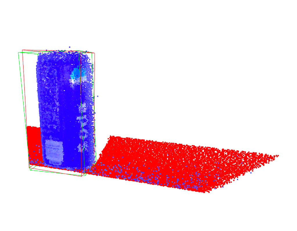
PCA is an important tool for dimensionality reduction in data science and to compute grasp poses for robotic manipulation from point cloud data. PCA can also directly used within a larger machine learning framework as it is differentiable. Using the two principal components of a point cloud for robotic grasping as an example, we will derive a numerical implementation of the PCA, which will help to understand what PCA is and what it does.
Principal Component Analysis (PCA) is widely used in data analysis and machine learning to reduce the dimensionality of a dataset. The goal is to find a set of linearly uncorrelated (orthogonal) variables, called principal components, that capture the maximum variance in the data. The first principal component represents the direction of maximum variance, the second principal component is orthogonal to the first and represents the direction of the next highest variance, and so on. PCA is also used in robotic manipulation to find the principal axis of a point cloud, which can then be used to orient a gripper.
Mathematically, the orthogonality of principal components is achieved by finding the eigenvectors of the covariance matrix of the original data. These eigenvectors form a set of orthogonal basis vectors, and the corresponding eigenvalues indicate the amount of variance captured by each principal component. The orthogonality property is essential for the interpretability and usefulness of the principal components in reducing dimensionality and capturing the key patterns in the data.
As you know, the sample variance of a set of data points is a measure of the spread or dispersion of the values. For a random variable X with n data points, the sample variance s² is calculated as:
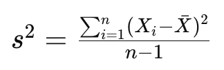
where barred X is the mean of the dataset. The division by n-1 instead of n is done to correct for bias in the estimation of the population variance when using a sample. This correction is known as Bessel’s correction and helps to provide an unbiased estimate of the population variance based on the sample data.
If we now assume our datapoints to be presented in an n-dimensional vector, X² will result in an nxn matrix. This is known as the sample covariance matrix. The covariance matrix is hence defined as

With this, we can implement this in Pytorch using its built-in PCA functions:
import torch
from sklearn.decomposition import PCA
from sklearn.datasets import make_blobs
import matplotlib.pyplot as plt

# Create synthetic data
data, labels = make_blobs(n_samples=100, n_features=2, centers=1,random_state=15)

# Convert NumPy array to PyTorch tensor
tensor_data = torch.from_numpy(data).float()

# Compute the mean of the data
mean = torch.mean(tensor_data, dim=0)

# Center the data by subtracting the mean
centered_data = tensor_data - mean

# Compute the covariance matrix
covariance_matrix = torch.mm(centered_data.t(), centered_data) / (tensor_data.size(0) - 1)

# Perform eigendecomposition of the covariance matrix
eigenvalues, eigenvectors = torch.linalg.eig(covariance_matrix)

# Sort eigenvalues and corresponding eigenvectors
sorted_indices = torch.argsort(eigenvalues.real, descending=True)
eigenvalues = eigenvalues[sorted_indices]
eigenvectors = eigenvectors[:, sorted_indices].to(centered_data.dtype)

# Pick the first two components
principal_components = eigenvectors[:, :2]*eigenvalues[:2].real

# Plot the original data with eigenvectors
plt.scatter(tensor_data[:, 0], tensor_data[:, 1], c=labels, cmap='viridis', label='Original Data')
plt.axis('equal')
plt.arrow(mean[0], mean[1], principal_components[0, 0], principal_components[1, 0], color='red', label='PC1')
plt.arrow(mean[0], mean[1], principal_components[0, 1], principal_components[1, 1], color='blue', label='PC2')

# Plot an ellipse around the Eigenvectors
angle = torch.atan2(principal_components[1,1],principal_components[0,1]).detach().numpy()/3.1415*180
ellipse=pat.Ellipse((mean[0].detach(), mean[1].detach()), 2*torch.norm(principal_components[:,1]), 2*torch.norm(principal_components[:,0]), angle=angle, fill=False)
ax = plt.gca()
ax.add_patch(ellipse)

plt.legend()
plt.show()
Note that the output of the PCA function is not necessarily sorted by the largest Eigenvalue. We are using the real part of each Eigenvalue for this and plot the resulting Eigenvectors below. Also note that we multiply each Eigenvector with the real part of its Eigenvalue to scale them.
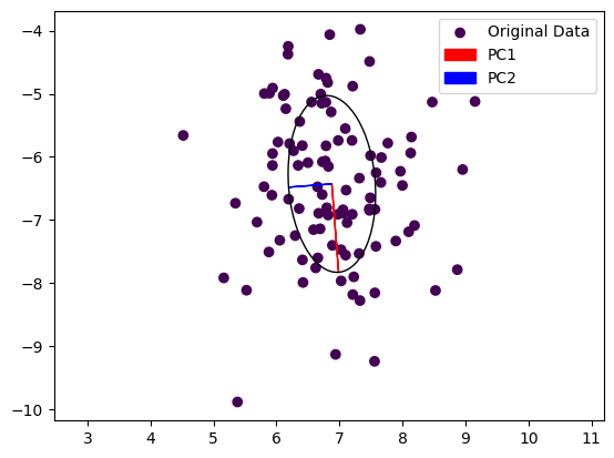
We can see that the first principal component, the dominant Eigenvector, is aligned with the longer axes of our random point cloud, whereas the second Eigenvector is aligned with the shorter axis. In a robotic application, we could now grasp this object by turning our gripper so that it is parallel to PC1 and close it along PC2. This of course works also in 3D, allowing us to also adjust the gripper’s pitch.
But what does the PCA function actually do? In practice, PCA is implemented using a singular value decomposition as solving the deterministic equation det(A−λI)=0 to find the Eigenvalues λ of a matrix A and hence computing the Eigenvectors might be infeasible. We will instead look at a simple numerical method to build some intution.
The Power Iteration method
The power iteration method is a simple and intuitive algorithm used to find the dominant eigenvector and eigenvalue of a square matrix. It’s particularly useful in the context of data science and machine learning when dealing with large, high-dimensional datasets, if only the first few Eigenvectors are needed.
An eigenvector is a non-zero vector that, when multiplied by a square matrix, results in a scaled version of the same vector. In other words, if A is a square matrix and v is a non-zero vector, then v is an eigenvector of A if there exists a scalar λ (called the eigenvalue) such that:
Av=λv
Here:
- A is the square matrix.
- v is the eigenvector.
- λ is the eigenvalue associated with the eigenvector v.
In other words, the matrix is reduced to a single number when multiplying its Eigenvectors. The power iteration method takes advantage of this by simply multiplying a random vector with A over and over again, and normalizing it.
Here’s a breakdown of the power iteration method:
- Initialization: Start with a random vector. This vector doesn’t need to have any specific properties; it’s just a starting point.
- Iterative Process:
– Multiply the matrix by the current vector. This results in a new vector.
– Normalize the new vector to have unit length (divide by its norm). - Convergence:
– Repeat the iterative process for a certain number of iterations or until the vector converges (stops changing significantly). - Result:
– The final vector is the dominant eigenvector.
– The corresponding eigenvalue is obtained by multiplying the transpose of the eigenvector with the original matrix and the eigenvector.
And here is the code:
def power_iteration(A, num_iterations=100):
    # 1. Initialize a random vector
    v = torch.randn(A.shape[1], 1, dtype=A.dtype)

    for _ in range(num_iterations):
        # 2. Multiply matrix by current vector and normalize
        v = torch.matmul(A, v)
        v /= torch.norm(v)
        # 3. Repeat

    # Compute the dominant eigenvalue
    eigenvalue = torch.matmul(torch.matmul(v.t(), A), v)

    return eigenvalue.item(), v.squeeze()

# Example: find the dominant eigenvector and Eigenvalue of a covariance matrix
dominant_eigenvalue, dominant_eigenvector = power_iteration(covariance_matrix)
In essence, the power iteration method leverages the repeated application of the matrix to a vector, causing the vector to align with the dominant eigenvector. It’s a straightforward and computationally efficient method, especially useful for large datasets where direct computation of eigenvectors may be impractical.
Computing the second Eigenvector using Gram-Schmidt Orthogonalization
Power iteration finds only the dominant eigenvector and eigenvalue. In order to find the next Eigenvector, we need to flatten the matrix. For this, we subtract the contribution of an Eigenvector from the original matrix:
A′=A−λvv^t
or in code:
def deflate_matrix(A, eigenvalue, eigenvector):
    deflated_matrix = A - eigenvalue * torch.matmul(eigenvector, eigenvector.t())
    return deflated_matrix
The purpose of obtaining a deflated matrix is to facilitate the iterative computation of subsequent eigenvalues and eigenvectors. After finding the first eigenvalue-eigenvector pair, you can use the deflated matrix to find the next one, and so on.
The result of this approach is not necessarily orthogonal, however. Gram-Schmidt orthogonalization is a process in linear algebra used to transform a set of linearly independent vectors into a set of orthogonal (perpendicular) vectors. This method is named after mathematicians Jørgen Gram and Erhard Schmidt and is particularly useful when working with non-orthogonal bases.
def gram_schmidt(v, u):
    # Gram-Schmidt orthogonalization
    projection = torch.matmul(u.t(), v) / torch.matmul(u.t(), u)
    v = v.squeeze(-1) - projection * u
    return v
- Input Parameters:
-v: The vector that you want to orthogonalize.
-u: The vector with respect to which you want to orthogonalize v. - Orthogonalization Step:
-torch.matmul(u.t(), v): This computes the dot product between u and v.
-torch.matmul(u.t(), u): This computes the dot product of u with itself (squared norm of u).
-projection = … / …: This calculates the scalar projection of v onto u. The projection is the amount of v that lies in the direction of u.
– v = v.squeeze(-1) – projection * u: This subtracts the projection of v onto u from v. The result is a new vector v that is orthogonal to u. - Return:
-The function returns the orthogonalized vector v.
We can now add Gram-Schmidt Orthogonalization to the Power Method and compute both the Dominant and the Second Eigenvector:
# Power iteration to find dominant eigenvector
dominant_eigenvalue, dominant_eigenvector = power_iteration(covariance_matrix)

deflated_matrix = deflate_matrix(covariance_matrix, dominant_eigenvalue, dominant_eigenvector)
second_eigenvector = deflated_matrix[:, 0].view(-1, 1)


# Power iteration to find the second eigenvector
for _ in range(100):
    second_eigenvector = torch.matmul(covariance_matrix, second_eigenvector)
    second_eigenvector /= torch.norm(second_eigenvector)
    # Orthogonalize with respect to the first eigenvector
    second_eigenvector = gram_schmidt(second_eigenvector, dominant_eigenvector)

second_eigenvalue = torch.matmul(torch.matmul(second_eigenvector.t(), covariance_matrix), second_eigenvector)
We can now plot the Eigenvectors computed with either method next to each other:
# Scale Eigenvectors by Eigenvalues
dominant_eigenvector *= dominant_eigenvalue
second_eigenvector *= second_eigenvalue

# Plot the original data with eigenvectors computed either way
plt.scatter(tensor_data[:, 0], tensor_data[:, 1], c=labels, cmap='viridis', label='Original Data')
plt.axis('equal')
plt.arrow(mean[0], mean[1], principal_components[0, 0], principal_components[1, 0], color='red', label='PC1')
plt.arrow(mean[0], mean[1], principal_components[0, 1], principal_components[1, 1], color='blue', label='PC2')
plt.arrow(mean[0], mean[1], dominant_eigenvector[0], dominant_eigenvector[1], color='orange', label='approx1')
plt.arrow(mean[0], mean[1], second_eigenvector[0], second_eigenvector[1], color='purple', label='approx2')
plt.legend()
plt.show()
…and the result is:
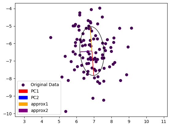
Note that the second Eigenvector coming from power iteration (purple) is painted over the second Eigenvector computed by the exact method (blue). The dominant Eigenvector from power iteration (yellow) is pointing in the other direction then the exact dominant Eigenvector (red). This is not really surprising, as we started from a random vector during power iteration and the result could come out either way.
Summary
We presented a simple numerical method to compute the Eigenvectors of a Covariance Matrix to derive the Principal Components of a dataset, shedding some light on the properties of Eigenvectors and Eigenvalues.
Understanding Principal Component Analysis in PyTorch was originally published in Towards Data Science on Medium, where people are continuing the conversation by highlighting and responding to this story.
Built-in function vs. numerical methods
PCA is an important tool for dimensionality reduction in data science and to compute grasp poses for robotic manipulation from point cloud data. PCA can also directly used within a larger machine learning framework as it is differentiable. Using the two principal components of a point cloud for robotic grasping as an example, we will derive a numerical implementation of the PCA, which will help to understand what PCA is and what it does.
Principal Component Analysis (PCA) is widely used in data analysis and machine learning to reduce the dimensionality of a dataset. The goal is to find a set of linearly uncorrelated (orthogonal) variables, called principal components, that capture the maximum variance in the data. The first principal component represents the direction of maximum variance, the second principal component is orthogonal to the first and represents the direction of the next highest variance, and so on. PCA is also used in robotic manipulation to find the principal axis of a point cloud, which can then be used to orient a gripper.
Mathematically, the orthogonality of principal components is achieved by finding the eigenvectors of the covariance matrix of the original data. These eigenvectors form a set of orthogonal basis vectors, and the corresponding eigenvalues indicate the amount of variance captured by each principal component. The orthogonality property is essential for the interpretability and usefulness of the principal components in reducing dimensionality and capturing the key patterns in the data.
As you know, the sample variance of a set of data points is a measure of the spread or dispersion of the values. For a random variable X with n data points, the sample variance s² is calculated as:
where barred X is the mean of the dataset. The division by n-1 instead of n is done to correct for bias in the estimation of the population variance when using a sample. This correction is known as Bessel’s correction and helps to provide an unbiased estimate of the population variance based on the sample data.
If we now assume our datapoints to be presented in an n-dimensional vector, X² will result in an nxn matrix. This is known as the sample covariance matrix. The covariance matrix is hence defined as
With this, we can implement this in Pytorch using its built-in PCA functions:
import torch
from sklearn.decomposition import PCA
from sklearn.datasets import make_blobs
import matplotlib.pyplot as plt

# Create synthetic data
data, labels = make_blobs(n_samples=100, n_features=2, centers=1,random_state=15)

# Convert NumPy array to PyTorch tensor
tensor_data = torch.from_numpy(data).float()

# Compute the mean of the data
mean = torch.mean(tensor_data, dim=0)

# Center the data by subtracting the mean
centered_data = tensor_data - mean

# Compute the covariance matrix
covariance_matrix = torch.mm(centered_data.t(), centered_data) / (tensor_data.size(0) - 1)

# Perform eigendecomposition of the covariance matrix
eigenvalues, eigenvectors = torch.linalg.eig(covariance_matrix)

# Sort eigenvalues and corresponding eigenvectors
sorted_indices = torch.argsort(eigenvalues.real, descending=True)
eigenvalues = eigenvalues[sorted_indices]
eigenvectors = eigenvectors[:, sorted_indices].to(centered_data.dtype)

# Pick the first two components
principal_components = eigenvectors[:, :2]*eigenvalues[:2].real

# Plot the original data with eigenvectors
plt.scatter(tensor_data[:, 0], tensor_data[:, 1], c=labels, cmap='viridis', label='Original Data')
plt.axis('equal')
plt.arrow(mean[0], mean[1], principal_components[0, 0], principal_components[1, 0], color='red', label='PC1')
plt.arrow(mean[0], mean[1], principal_components[0, 1], principal_components[1, 1], color='blue', label='PC2')

# Plot an ellipse around the Eigenvectors
angle = torch.atan2(principal_components[1,1],principal_components[0,1]).detach().numpy()/3.1415*180
ellipse=pat.Ellipse((mean[0].detach(), mean[1].detach()), 2*torch.norm(principal_components[:,1]), 2*torch.norm(principal_components[:,0]), angle=angle, fill=False)
ax = plt.gca()
ax.add_patch(ellipse)

plt.legend()
plt.show()
Note that the output of the PCA function is not necessarily sorted by the largest Eigenvalue. We are using the real part of each Eigenvalue for this and plot the resulting Eigenvectors below. Also note that we multiply each Eigenvector with the real part of its Eigenvalue to scale them.
We can see that the first principal component, the dominant Eigenvector, is aligned with the longer axes of our random point cloud, whereas the second Eigenvector is aligned with the shorter axis. In a robotic application, we could now grasp this object by turning our gripper so that it is parallel to PC1 and close it along PC2. This of course works also in 3D, allowing us to also adjust the gripper’s pitch.
But what does the PCA function actually do? In practice, PCA is implemented using a singular value decomposition as solving the deterministic equation det(A−λI)=0 to find the Eigenvalues λ of a matrix A and hence computing the Eigenvectors might be infeasible. We will instead look at a simple numerical method to build some intution.
The Power Iteration method
The power iteration method is a simple and intuitive algorithm used to find the dominant eigenvector and eigenvalue of a square matrix. It’s particularly useful in the context of data science and machine learning when dealing with large, high-dimensional datasets, if only the first few Eigenvectors are needed.
An eigenvector is a non-zero vector that, when multiplied by a square matrix, results in a scaled version of the same vector. In other words, if A is a square matrix and v is a non-zero vector, then v is an eigenvector of A if there exists a scalar λ (called the eigenvalue) such that:
Av=λv
Here:
- A is the square matrix.
- v is the eigenvector.
- λ is the eigenvalue associated with the eigenvector v.
In other words, the matrix is reduced to a single number when multiplying its Eigenvectors. The power iteration method takes advantage of this by simply multiplying a random vector with A over and over again, and normalizing it.
Here’s a breakdown of the power iteration method:
- Initialization: Start with a random vector. This vector doesn’t need to have any specific properties; it’s just a starting point.
- Iterative Process:
– Multiply the matrix by the current vector. This results in a new vector.
– Normalize the new vector to have unit length (divide by its norm). - Convergence:
– Repeat the iterative process for a certain number of iterations or until the vector converges (stops changing significantly). - Result:
– The final vector is the dominant eigenvector.
– The corresponding eigenvalue is obtained by multiplying the transpose of the eigenvector with the original matrix and the eigenvector.
And here is the code:
def power_iteration(A, num_iterations=100):
    # 1. Initialize a random vector
    v = torch.randn(A.shape[1], 1, dtype=A.dtype)

    for _ in range(num_iterations):
        # 2. Multiply matrix by current vector and normalize
        v = torch.matmul(A, v)
        v /= torch.norm(v)
        # 3. Repeat

    # Compute the dominant eigenvalue
    eigenvalue = torch.matmul(torch.matmul(v.t(), A), v)

    return eigenvalue.item(), v.squeeze()

# Example: find the dominant eigenvector and Eigenvalue of a covariance matrix
dominant_eigenvalue, dominant_eigenvector = power_iteration(covariance_matrix)
In essence, the power iteration method leverages the repeated application of the matrix to a vector, causing the vector to align with the dominant eigenvector. It’s a straightforward and computationally efficient method, especially useful for large datasets where direct computation of eigenvectors may be impractical.
Computing the second Eigenvector using Gram-Schmidt Orthogonalization
Power iteration finds only the dominant eigenvector and eigenvalue. In order to find the next Eigenvector, we need to flatten the matrix. For this, we subtract the contribution of an Eigenvector from the original matrix:
A′=A−λvv^t
or in code:
def deflate_matrix(A, eigenvalue, eigenvector):
    deflated_matrix = A - eigenvalue * torch.matmul(eigenvector, eigenvector.t())
    return deflated_matrix
The purpose of obtaining a deflated matrix is to facilitate the iterative computation of subsequent eigenvalues and eigenvectors. After finding the first eigenvalue-eigenvector pair, you can use the deflated matrix to find the next one, and so on.
The result of this approach is not necessarily orthogonal, however. Gram-Schmidt orthogonalization is a process in linear algebra used to transform a set of linearly independent vectors into a set of orthogonal (perpendicular) vectors. This method is named after mathematicians Jørgen Gram and Erhard Schmidt and is particularly useful when working with non-orthogonal bases.
def gram_schmidt(v, u):
    # Gram-Schmidt orthogonalization
    projection = torch.matmul(u.t(), v) / torch.matmul(u.t(), u)
    v = v.squeeze(-1) - projection * u
    return v
- Input Parameters:
-v: The vector that you want to orthogonalize.
-u: The vector with respect to which you want to orthogonalize v. - Orthogonalization Step:
-torch.matmul(u.t(), v): This computes the dot product between u and v.
-torch.matmul(u.t(), u): This computes the dot product of u with itself (squared norm of u).
-projection = … / …: This calculates the scalar projection of v onto u. The projection is the amount of v that lies in the direction of u.
– v = v.squeeze(-1) – projection * u: This subtracts the projection of v onto u from v. The result is a new vector v that is orthogonal to u. - Return:
-The function returns the orthogonalized vector v.
We can now add Gram-Schmidt Orthogonalization to the Power Method and compute both the Dominant and the Second Eigenvector:
# Power iteration to find dominant eigenvector
dominant_eigenvalue, dominant_eigenvector = power_iteration(covariance_matrix)

deflated_matrix = deflate_matrix(covariance_matrix, dominant_eigenvalue, dominant_eigenvector)
second_eigenvector = deflated_matrix[:, 0].view(-1, 1)


# Power iteration to find the second eigenvector
for _ in range(100):
    second_eigenvector = torch.matmul(covariance_matrix, second_eigenvector)
    second_eigenvector /= torch.norm(second_eigenvector)
    # Orthogonalize with respect to the first eigenvector
    second_eigenvector = gram_schmidt(second_eigenvector, dominant_eigenvector)

second_eigenvalue = torch.matmul(torch.matmul(second_eigenvector.t(), covariance_matrix), second_eigenvector)
We can now plot the Eigenvectors computed with either method next to each other:
# Scale Eigenvectors by Eigenvalues
dominant_eigenvector *= dominant_eigenvalue
second_eigenvector *= second_eigenvalue

# Plot the original data with eigenvectors computed either way
plt.scatter(tensor_data[:, 0], tensor_data[:, 1], c=labels, cmap='viridis', label='Original Data')
plt.axis('equal')
plt.arrow(mean[0], mean[1], principal_components[0, 0], principal_components[1, 0], color='red', label='PC1')
plt.arrow(mean[0], mean[1], principal_components[0, 1], principal_components[1, 1], color='blue', label='PC2')
plt.arrow(mean[0], mean[1], dominant_eigenvector[0], dominant_eigenvector[1], color='orange', label='approx1')
plt.arrow(mean[0], mean[1], second_eigenvector[0], second_eigenvector[1], color='purple', label='approx2')
plt.legend()
plt.show()
…and the result is:
Note that the second Eigenvector coming from power iteration (purple) is painted over the second Eigenvector computed by the exact method (blue). The dominant Eigenvector from power iteration (yellow) is pointing in the other direction then the exact dominant Eigenvector (red). This is not really surprising, as we started from a random vector during power iteration and the result could come out either way.
Summary
We presented a simple numerical method to compute the Eigenvectors of a Covariance Matrix to derive the Principal Components of a dataset, shedding some light on the properties of Eigenvectors and Eigenvalues.
Understanding Principal Component Analysis in PyTorch was originally published in Towards Data Science on Medium, where people are continuing the conversation by highlighting and responding to this story.
Denial of responsibility! Techno Blender is an automatic aggregator of the all world’s media. In each content, the hyperlink to the primary source is specified. All trademarks belong to their rightful owners, all materials to their authors. If you are the owner of the content and do not want us to publish your materials, please contact us by email – [email protected]. The content will be deleted within 24 hours.