Vision Transformers, Explained

By Jessie Hobb On Feb 27, 2024

Vision Transformers Explained Series

A Full Walk-Through of Vision Transformers in PyTorch

Since their introduction in 2017 with Attention is All You Need¹, transformers have established themselves as the state of the art for natural language processing (NLP). In 2021, An Image is Worth 16×16 Words² successfully adapted transformers for computer vision tasks. Since then, numerous transformer-based architectures have been proposed for computer vision.

This article walks through the Vision Transformer (ViT) as laid out in An Image is Worth 16×16 Words². It includes open-source code for the ViT, as well as conceptual explanations of the components. All of the code uses the PyTorch Python package.

Photo by Sahand Babali on Unsplash

This article is part of a collection examining the internal workings of Vision Transformers in depth. Each of these articles is also available as a Jupyter Notebook with executable code. The other articles in the series are:

Vision Transformers, Explained
→ Jupyter Notebook
Attention for Vision Transformers, Explained
→ Jupyter Notebook
Position Embeddings for Vision Transformers, Explained
→ Jupyter Notebook
Tokens-to-Token Vision Transformers, Explained
→ Jupyter Notebook
GitHub Repository for Vision Transformers, Explained Series

What Are Vision Transformers?
Model Walk-Through
— Image Tokenization
— Token Processing
— Encoding Block
— Neural Network Module
— Prediction Processing
Complete Code
Conclusion
— Further Reading
— Citations

What are Vision Transformers?

As introduced in Attention is All You Need¹, transformers are a type of machine learning model utilizing attention as the primary learning mechanism. Transformers quickly became the state of the art for sequence-to-sequence tasks such as language translation.

An Image is Worth 16×16 Words² successfully modified the transformer put forth in [1] to solve image classification tasks, creating the Vision Transformer (ViT). The ViT is based on the same attention mechanism as the transformer in [1]. However, while transformers for NLP tasks consist of an encoder attention branch and a decoder attention branch, the ViT only uses an encoder. The output of the encoder is then passed to a neural network “head” that makes a prediction.

The drawback of ViT as implemented in [2] is that it’s optimal performance requires pretraining on large datasets. The best models pretrained on the proprietary JFT-300M dataset. Models pretrained on the smaller, open source ImageNet-21k perform on par with the state-of-the-art convolutional ResNet models.

Tokens-to-Token ViT: Training Vision Transformers from Scratch on ImageNet³ attempts to remove this pretraining requirement by introducing a novel pre-processing methodology to transform an input image into a series of tokens. More about this method can be found here. For this article, we’ll focus on the ViT as implemented in [2].

Model Walk-Through

This article follows the model structure outlined in An Image is Worth 16×16 Words². However, code from this paper is not publicly available. Code from the more recent Tokens-to-Token ViT³ is available on GitHub. The Tokens-to-Token ViT (T2T-ViT) model prepends a Tokens-to-Token (T2T) module to a vanilla ViT backbone. The code in this article is based on the ViT components in the Tokens-to-Token ViT³ GitHub code. Modifications made for this article include, but are not limited to, modifying to allow for non-square input images and removing dropout layers.

A diagram of the ViT model is shown below.

Image Tokenization

The first step of the ViT is to create tokens from the input image. Transformers operate on a sequence of tokens; in NLP, this is commonly a sentence of words. For computer vision, it is less clear how to segment the input into tokens.

The ViT converts an image to tokens such that each token represents a local area — or patch — of the image. They describe reshaping an image of height H, width W, and channels C into N tokens with patch size P:

https://medium.com/media/8ccfff44b75b89da6fad4a44f6a6828e/href

Each token is of length P²∗C.

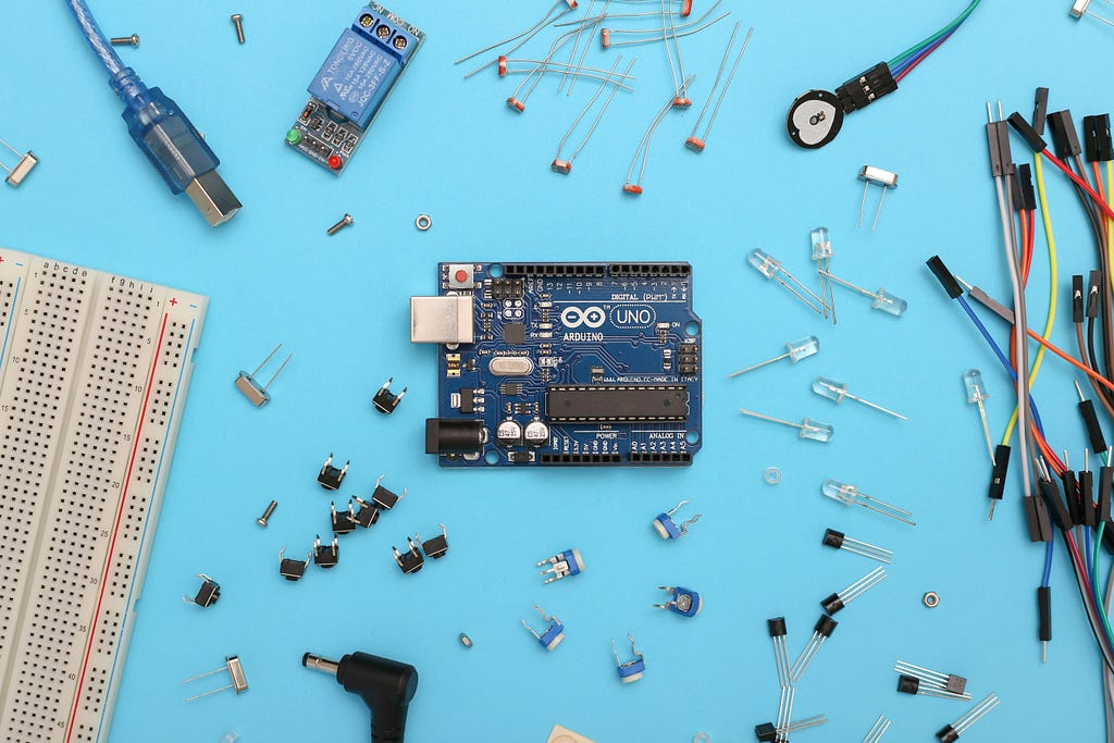
Let’s look at an example of patch tokenization on this pixel art Mountain at Dusk by Luis Zuno (@ansimuz)⁴. The original artwork has been cropped and converted to a single channel image. This means that each pixel has a value between zero and one. Single channel images are typically displayed in grayscale; however, we’ll be displaying it in a purple color scheme because its easier to see.

Note that the patch tokenization is not included in the code associated with [3]. All code in this section is original to the author.

mountains = np.load(os.path.join(figure_path, 'mountains.npy'))

H = mountains.shape[0]
W = mountains.shape[1]
print('Mountain at Dusk is H =', H, 'and W =', W, 'pixels.')
print('\n')

fig = plt.figure(figsize=(10,6))
plt.imshow(mountains, cmap='Purples_r')
plt.xticks(np.arange(-0.5, W+1, 10), labels=np.arange(0, W+1, 10))
plt.yticks(np.arange(-0.5, H+1, 10), labels=np.arange(0, H+1, 10))
plt.clim([0,1])
cbar_ax = fig.add_axes([0.95, .11, 0.05, 0.77])
plt.clim([0, 1])
plt.colorbar(cax=cbar_ax);
#plt.savefig(os.path.join(figure_path, 'mountains.png'))

Mountain at Dusk is H = 60 and W = 100 pixels.

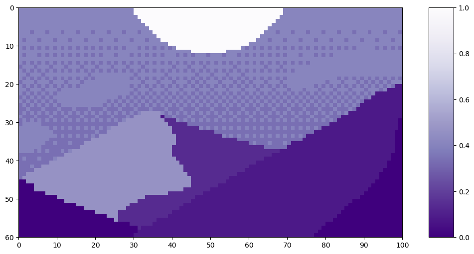
This image has H=60 and W=100. We’ll set P=20 since it divides both H and W evenly.

P = 20
N = int((H*W)/(P**2))
print('There will be', N, 'patches, each', P, 'by', str(P)+'.')
print('\n')

fig = plt.figure(figsize=(10,6))
plt.imshow(mountains, cmap='Purples_r')
plt.hlines(np.arange(P, H, P)-0.5, -0.5, W-0.5, color='w')
plt.vlines(np.arange(P, W, P)-0.5, -0.5, H-0.5, color='w')
plt.xticks(np.arange(-0.5, W+1, 10), labels=np.arange(0, W+1, 10))
plt.yticks(np.arange(-0.5, H+1, 10), labels=np.arange(0, H+1, 10))
x_text = np.tile(np.arange(9.5, W, P), 3)
y_text = np.repeat(np.arange(9.5, H, P), 5)
for i in range(1, N+1):
    plt.text(x_text[i-1], y_text[i-1], str(i), color='w', fontsize='xx-large', ha='center')
plt.text(x_text[2], y_text[2], str(3), color='k', fontsize='xx-large', ha='center');
#plt.savefig(os.path.join(figure_path, 'mountain_patches.png'), bbox_inches='tight'

There will be 15 patches, each 20 by 20.

By flattening these patches, we see the resulting tokens. Let’s look at patch 12 as an example, since it has four different shades in it.

print('Each patch will make a token of length', str(P**2)+'.')
print('\n')

patch12 = mountains[40:60, 20:40]
token12 = patch12.reshape(1, P**2)

fig = plt.figure(figsize=(10,1))
plt.imshow(token12, aspect=10, cmap='Purples_r')
plt.clim([0,1])
plt.xticks(np.arange(-0.5, 401, 50), labels=np.arange(0, 401, 50))
plt.yticks([]);
#plt.savefig(os.path.join(figure_path, 'mountain_token12.png'), bbox_inches='tight')

Each patch will make a token of length 400.

After extracting tokens from an image, it is common to use a linear projection to change the length of the tokens. This is implemented as a learnable linear layer. The new length of the tokens is referred to as the latent dimension², channel dimension³, or the token length. After the projection, the tokens are no longer visually identifiable as a patch from the original image.

Now that we understand the concept, we can look at how patch tokenization is implemented in code.

class Patch_Tokenization(nn.Module):
    def __init__(self,
                img_size: tuple[int, int, int]=(1, 1, 60, 100),
                patch_size: int=50,
                token_len: int=768):

        """ Patch Tokenization Module
            Args:
                img_size (tuple[int, int, int]): size of input (channels, height, width)
                patch_size (int): the side length of a square patch
                token_len (int): desired length of an output token
        """
        super().__init__()

        ## Defining Parameters
        self.img_size = img_size
        C, H, W = self.img_size
        self.patch_size = patch_size
        self.token_len = token_len
        assert H % self.patch_size == 0, 'Height of image must be evenly divisible by patch size.'
        assert W % self.patch_size == 0, 'Width of image must be evenly divisible by patch size.'
        self.num_tokens = (H / self.patch_size) * (W / self.patch_size)

        ## Defining Layers
        self.split = nn.Unfold(kernel_size=self.patch_size, stride=self.patch_size, padding=0)
        self.project = nn.Linear((self.patch_size**2)*C, token_len)

    def forward(self, x):
        x = self.split(x).transpose(1,0)
        x = self.project(x)
        return x

Note the two assert statements that ensure the image dimensions are evenly divisible by the patch size. The actual splitting into patches is implemented as a torch.nn.Unfold⁵ layer.

We’ll run an example of this code using our cropped, single channel version of Mountain at Dusk⁴. We should see the values for number of tokens and initial token size as we did above. We’ll use token_len=768 as the projected length, which is the size for the base variant of ViT².

The first line in the code block below is changing the datatype of Mountain at Dusk⁴ from a NumPy array to a Torch tensor. We also have to unsqueeze⁶ the tensor to create a channel dimension and a batch size dimension. As above, we have one channel. Since there is only one image, batchsize=1.

x = torch.from_numpy(mountains).unsqueeze(0).unsqueeze(0).to(torch.float32)
token_len = 768
print('Input dimensions are\n\tbatchsize:', x.shape[0], '\n\tnumber of input channels:', x.shape[1], '\n\timage size:', (x.shape[2], x.shape[3]))

# Define the Module
patch_tokens = Patch_Tokenization(img_size=(x.shape[1], x.shape[2], x.shape[3]),
                                    patch_size = P,
                                    token_len = token_len)

Input dimensions are
   batchsize: 1 
   number of input channels: 1 
   image size: (60, 100)

Now, we’ll split the image into tokens.

x = patch_tokens.split(x).transpose(2,1)
print('After patch tokenization, dimensions are\n\tbatchsize:', x.shape[0], '\n\tnumber of tokens:', x.shape[1], '\n\ttoken length:', x.shape[2])

After patch tokenization, dimensions are
   batchsize: 1 
   number of tokens: 15 
   token length: 400

As we saw in the example, there are N=15 tokens each of length 400. Lastly, we project the tokens to be the token_len.

x = patch_tokens.project(x)
print('After projection, dimensions are\n\tbatchsize:', x.shape[0], '\n\tnumber of tokens:', x.shape[1], '\n\ttoken length:', x.shape[2])

After projection, dimensions are
   batchsize: 1 
   number of tokens: 15 
   token length: 768

Now that we have tokens, we’re ready to proceed through the ViT.

Token Processing

We’ll designate the next two steps of the ViT, before the encoding blocks, as “token processing.” The token processing component of the ViT diagram is shown below.

The first step is to prepend a blank token, called the Prediction Token, to the the image tokens. This token will be used at the output of the encoding blocks to make a prediction. It starts off blank — equivalently zero — so that it can gain information from the other image tokens.

We’ll be starting with 175 tokens. Each token has length 768, which is the size for the base variant of ViT². We’re using a batch size of 13 because it’s prime and won’t be confused for any of the other parameters.

# Define an Input
num_tokens = 175
token_len = 768
batch = 13
x = torch.rand(batch, num_tokens, token_len)
print('Input dimensions are\n\tbatchsize:', x.shape[0], '\n\tnumber of tokens:', x.shape[1], '\n\ttoken length:', x.shape[2])

# Append a Prediction Token
pred_token = torch.zeros(1, 1, token_len).expand(batch, -1, -1)
print('Prediction Token dimensions are\n\tbatchsize:', pred_token.shape[0], '\n\tnumber of tokens:', pred_token.shape[1], '\n\ttoken length:', pred_token.shape[2])

x = torch.cat((pred_token, x), dim=1)
print('Dimensions with Prediction Token are\n\tbatchsize:', x.shape[0], '\n\tnumber of tokens:', x.shape[1], '\n\ttoken length:', x.shape[2])

Input dimensions are
   batchsize: 13 
   number of tokens: 175 
   token length: 768
Prediction Token dimensions are
   batchsize: 13 
   number of tokens: 1 
   token length: 768
Dimensions with Prediction Token are
   batchsize: 13 
   number of tokens: 176 
   token length: 768

Now, we add a position embedding for our tokens. The position embedding allows the transformer to understand the order of the image tokens. Note that this is an addition, not a concatenation. The specifics of position embeddings are a tangent best left for another time.

def get_sinusoid_encoding(num_tokens, token_len):
    """ Make Sinusoid Encoding Table

        Args:
            num_tokens (int): number of tokens
            token_len (int): length of a token
            
        Returns:
            (torch.FloatTensor) sinusoidal position encoding table
    """

    def get_position_angle_vec(i):
        return [i / np.power(10000, 2 * (j // 2) / token_len) for j in range(token_len)]

    sinusoid_table = np.array([get_position_angle_vec(i) for i in range(num_tokens)])
    sinusoid_table[:, 0::2] = np.sin(sinusoid_table[:, 0::2])
    sinusoid_table[:, 1::2] = np.cos(sinusoid_table[:, 1::2]) 

    return torch.FloatTensor(sinusoid_table).unsqueeze(0)

PE = get_sinusoid_encoding(num_tokens+1, token_len)
print('Position embedding dimensions are\n\tnumber of tokens:', PE.shape[1], '\n\ttoken length:', PE.shape[2])

x = x + PE
print('Dimensions with Position Embedding are\n\tbatchsize:', x.shape[0], '\n\tnumber of tokens:', x.shape[1], '\n\ttoken length:', x.shape[2])

Position embedding dimensions are
   number of tokens: 176 
   token length: 768
Dimensions with Position Embedding are
   batchsize: 13 
   number of tokens: 176 
   token length: 768

Now, our tokens are ready to proceed to the encoding blocks.

Encoding Block

The encoding block is where the model actually learns from the image tokens. The number of encoding blocks is a hyperparameter set by the user. A diagram of the encoding block is below.

The code for an encoding block is below.

class Encoding(nn.Module):

    def __init__(self,
       dim: int,
       num_heads: int=1,
       hidden_chan_mul: float=4.,
       qkv_bias: bool=False,
       qk_scale: NoneFloat=None,
       act_layer=nn.GELU, 
       norm_layer=nn.LayerNorm):
        
        """ Encoding Block

            Args:
                dim (int): size of a single token
                num_heads(int): number of attention heads in MSA
                hidden_chan_mul (float): multiplier to determine the number of hidden channels (features) in the NeuralNet component
                qkv_bias (bool): determines if the qkv layer learns an addative bias
                qk_scale (NoneFloat): value to scale the queries and keys by; 
                                    if None, queries and keys are scaled by ``head_dim ** -0.5``
                act_layer(nn.modules.activation): torch neural network layer class to use as activation
                norm_layer(nn.modules.normalization): torch neural network layer class to use as normalization
        """

        super().__init__()

        ## Define Layers
        self.norm1 = norm_layer(dim)
        self.attn = Attention(dim=dim,
                            chan=dim,
                            num_heads=num_heads,
                            qkv_bias=qkv_bias,
                            qk_scale=qk_scale)
        self.norm2 = norm_layer(dim)
        self.neuralnet = NeuralNet(in_chan=dim,
                                hidden_chan=int(dim*hidden_chan_mul),
                                out_chan=dim,
                                act_layer=act_layer)

    def forward(self, x):
        x = x + self.attn(self.norm1(x))
        x = x + self.neuralnet(self.norm2(x))
        return x

The num_heads, qkv_bias, and qk_scale parameters define the Attention module components. A deep dive into attention for vision transformers is left for another time.

The hidden_chan_mul and act_layer parameters define the Neural Network module components. The activation layer can be any torch.nn.modules.activation⁷ layer. We’ll look more at the Neural Network module later.

The norm_layer can be chosen from any torch.nn.modules.normalization⁸ layer.

We’ll now step through each blue block in the diagram and its accompanying code. We’ll use 176 tokens of length 768. We’ll use a batch size of 13 because it’s prime and won’t be confused for any of the other parameters. We’ll use 4 attention heads because it evenly divides token length; however, you won’t see the attention head dimension in the encoding block.

# Define an Input
num_tokens = 176
token_len = 768
batch = 13
heads = 4
x = torch.rand(batch, num_tokens, token_len)
print('Input dimensions are\n\tbatchsize:', x.shape[0], '\n\tnumber of tokens:', x.shape[1], '\n\ttoken length:', x.shape[2])

# Define the Module
E = Encoding(dim=token_len, num_heads=heads, hidden_chan_mul=1.5, qkv_bias=False, qk_scale=None, act_layer=nn.GELU, norm_layer=nn.LayerNorm)
E.eval();

Input dimensions are
   batchsize: 13 
   number of tokens: 176 
   token length: 768

Now, we’ll pass through a norm layer and an Attention module. The Attention module in the encoding block is parameterized so that it don’t change the token length. After the Attention module, we implement our first split connection.

y = E.norm1(x)
print('After norm, dimensions are\n\tbatchsize:', y.shape[0], '\n\tnumber of tokens:', y.shape[1], '\n\ttoken size:', y.shape[2])
y = E.attn(y)
print('After attention, dimensions are\n\tbatchsize:', y.shape[0], '\n\tnumber of tokens:', y.shape[1], '\n\ttoken size:', y.shape[2])
y = y + x
print('After split connection, dimensions are\n\tbatchsize:', y.shape[0], '\n\tnumber of tokens:', y.shape[1], '\n\ttoken size:', y.shape[2])

After norm, dimensions are
   batchsize: 13 
   number of tokens: 176 
   token size: 768
After attention, dimensions are
   batchsize: 13 
   number of tokens: 176 
   token size: 768
After split connection, dimensions are
   batchsize: 13 
   number of tokens: 176 
   token size: 768

Now, we pass through another norm layer, and then the Neural Network module. We finish with the second split connection.

z = E.norm2(y)
print('After norm, dimensions are\n\tbatchsize:', z.shape[0], '\n\tnumber of tokens:', z.shape[1], '\n\ttoken size:', z.shape[2])
z = E.neuralnet(z)
print('After neural net, dimensions are\n\tbatchsize:', z.shape[0], '\n\tnumber of tokens:', z.shape[1], '\n\ttoken size:', z.shape[2])
z = z + y
print('After split connection, dimensions are\n\tbatchsize:', z.shape[0], '\n\tnumber of tokens:', z.shape[1], '\n\ttoken size:', z.shape[2])

After norm, dimensions are
   batchsize: 13 
   number of tokens: 176 
   token size: 768
After neural net, dimensions are
   batchsize: 13 
   number of tokens: 176 
   token size: 768
After split connection, dimensions are
   batchsize: 13 
   number of tokens: 176 
   token size: 768

That’s all for a single encoding block! Since the final dimensions are the same as the initial dimensions, the model can easily pass tokens through multiple encoding blocks, as set by the depth hyperparameter.

Neural Network Module

The Neural Network (NN) module is a sub-component of the encoding block. The NN module is very simple, consisting of a fully-connected layer, an activation layer, and another fully-connected layer. The activation layer can be any torch.nn.modules.activation⁷ layer, which is passed as input to the module. The NN module can be configured to change the shape of an input, or to maintain the same shape. We’re not going to step through this code, as neural networks are common in machine learning, and not the focus of this article. However, the code for the NN module is presented below.

class NeuralNet(nn.Module):
    def __init__(self,
       in_chan: int,
       hidden_chan: NoneFloat=None,
       out_chan: NoneFloat=None,
       act_layer = nn.GELU):
        """ Neural Network Module

            Args:
                in_chan (int): number of channels (features) at input
                hidden_chan (NoneFloat): number of channels (features) in the hidden layer;
                                        if None, number of channels in hidden layer is the same as the number of input channels
                out_chan (NoneFloat): number of channels (features) at output;
                                        if None, number of output channels is same as the number of input channels
                act_layer(nn.modules.activation): torch neural network layer class to use as activation
        """

        super().__init__()

        ## Define Number of Channels
        hidden_chan = hidden_chan or in_chan
        out_chan = out_chan or in_chan

        ## Define Layers
        self.fc1 = nn.Linear(in_chan, hidden_chan)
        self.act = act_layer()
        self.fc2 = nn.Linear(hidden_chan, out_chan)

    def forward(self, x):
        x = self.fc1(x)
        x = self.act(x)
        x = self.fc2(x)
        return x

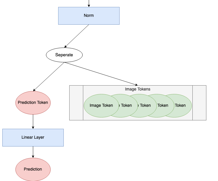
Prediction Processing

After passing through the encoding blocks, the last thing the model must do is make a prediction. The “prediction processing” component of the ViT diagram is shown below.

We’re going to look at each step of this process. We’ll continue with 176 tokens of length 768. We’ll use a batch size of 1 to illustrate how a single prediction is made. A batch size greater than 1 would be computing this prediction in parallel.

# Define an Input
num_tokens = 176
token_len = 768
batch = 1
x = torch.rand(batch, num_tokens, token_len)
print('Input dimensions are\n\tbatchsize:', x.shape[0], '\n\tnumber of tokens:', x.shape[1], '\n\ttoken length:', x.shape[2])

Input dimensions are
   batchsize: 1 
   number of tokens: 176 
   token length: 768

First, all the tokens are passed through a norm layer.

norm = nn.LayerNorm(token_len)
x = norm(x)
print('After norm, dimensions are\n\tbatchsize:', x.shape[0], '\n\tnumber of tokens:', x.shape[1], '\n\ttoken size:', x.shape[2])

After norm, dimensions are
   batchsize: 1 
   number of tokens: 1001 
   token size: 768

Next, we split off the prediction token from the rest of the tokens. Throughout the encoding block(s), the prediction token has become nonzero and gained information about our input image. We’ll use only this prediction token to make a final prediction.

pred_token = x[:, 0]
print('Length of prediction token:', pred_token.shape[-1])

Length of prediction token: 768

Finally, the prediction token is passed through the head to make a prediction. The head, usually some variety of neural network, is varied based on the model. In An Image is Worth 16×16 Words², they use an MLP (multilayer perceptron) with one hidden layer during pretraining and a single linear layer during fine tuning. In Tokens-to-Token ViT³, they use a single linear layer as a head. This example proceeds with a single linear layer.

Note that the output shape of the head is set based on the parameters of the learning problem. For classification, it is typically a vector of length number of classes in a one-hot encoding. For regression, it would be any integer number of predicted parameters. This example will use an output shape of 1 to represent a single estimated regression value.

head = nn.Linear(token_len, 1)
pred = head(pred_token)
print('Length of prediction:', (pred.shape[0], pred.shape[1]))
print('Prediction:', float(pred))

Length of prediction: (1, 1)
Prediction: -0.5474240779876709

And that’s all! The model has made a prediction!

Complete Code

To create the complete ViT module, we use the Patch Tokenization module defined above and the ViT Backbone module. The ViT Backbone is defined below, and contains the Token Processing, Encoding Blocks, and Prediction Processing components.

class ViT_Backbone(nn.Module):
    def __init__(self,
                preds: int=1,
                token_len: int=768,
                num_heads: int=1,
                Encoding_hidden_chan_mul: float=4.,
                depth: int=12,
                qkv_bias=False,
                qk_scale=None,
                act_layer=nn.GELU,
                norm_layer=nn.LayerNorm):

        """ VisTransformer Backbone
            Args:
                preds (int): number of predictions to output
                token_len (int): length of a token
                num_heads(int): number of attention heads in MSA
                Encoding_hidden_chan_mul (float): multiplier to determine the number of hidden channels (features) in the NeuralNet component of the Encoding Module
                depth (int): number of encoding blocks in the model
                qkv_bias (bool): determines if the qkv layer learns an addative bias
                qk_scale (NoneFloat): value to scale the queries and keys by; 
                 if None, queries and keys are scaled by ``head_dim ** -0.5``
                act_layer(nn.modules.activation): torch neural network layer class to use as activation
                norm_layer(nn.modules.normalization): torch neural network layer class to use as normalization
        """

        super().__init__()

        ## Defining Parameters
        self.num_heads = num_heads
        self.Encoding_hidden_chan_mul = Encoding_hidden_chan_mul
        self.depth = depth

        ## Defining Token Processing Components
        self.cls_token = nn.Parameter(torch.zeros(1, 1, self.token_len))
        self.pos_embed = nn.Parameter(data=get_sinusoid_encoding(num_tokens=self.num_tokens+1, token_len=self.token_len), requires_grad=False)

        ## Defining Encoding blocks
        self.blocks = nn.ModuleList([Encoding(dim = self.token_len, 
                                               num_heads = self.num_heads,
                                               hidden_chan_mul = self.Encoding_hidden_chan_mul,
                                               qkv_bias = qkv_bias,
                                               qk_scale = qk_scale,
                                               act_layer = act_layer,
                                               norm_layer = norm_layer)
             for i in range(self.depth)])

        ## Defining Prediction Processing
        self.norm = norm_layer(self.token_len)
        self.head = nn.Linear(self.token_len, preds)

        ## Make the class token sampled from a truncated normal distrobution 
        timm.layers.trunc_normal_(self.cls_token, std=.02)

    def forward(self, x):
        ## Assumes x is already tokenized

        ## Get Batch Size
        B = x.shape[0]
        ## Concatenate Class Token
        x = torch.cat((self.cls_token.expand(B, -1, -1), x), dim=1)
        ## Add Positional Embedding
        x = x + self.pos_embed
        ## Run Through Encoding Blocks
        for blk in self.blocks:
            x = blk(x)
        ## Take Norm
        x = self.norm(x)
        ## Make Prediction on Class Token
        x = self.head(x[:, 0])
        return x

From the ViT Backbone module, we can define the full ViT model.

class ViT_Model(nn.Module):
 def __init__(self,
    img_size: tuple[int, int, int]=(1, 400, 100),
    patch_size: int=50,
    token_len: int=768,
    preds: int=1,
    num_heads: int=1,
    Encoding_hidden_chan_mul: float=4.,
    depth: int=12,
    qkv_bias=False,
    qk_scale=None,
    act_layer=nn.GELU,
    norm_layer=nn.LayerNorm):

  """ VisTransformer Model

   Args:
    img_size (tuple[int, int, int]): size of input (channels, height, width)
    patch_size (int): the side length of a square patch
    token_len (int): desired length of an output token
    preds (int): number of predictions to output
    num_heads(int): number of attention heads in MSA
    Encoding_hidden_chan_mul (float): multiplier to determine the number of hidden channels (features) in the NeuralNet component of the Encoding Module
    depth (int): number of encoding blocks in the model
    qkv_bias (bool): determines if the qkv layer learns an addative bias
    qk_scale (NoneFloat): value to scale the queries and keys by; 
         if None, queries and keys are scaled by ``head_dim ** -0.5``
    act_layer(nn.modules.activation): torch neural network layer class to use as activation
    norm_layer(nn.modules.normalization): torch neural network layer class to use as normalization
  """
  super().__init__()

  ## Defining Parameters
  self.img_size = img_size
  C, H, W = self.img_size
  self.patch_size = patch_size
  self.token_len = token_len
  self.num_heads = num_heads
  self.Encoding_hidden_chan_mul = Encoding_hidden_chan_mul
  self.depth = depth

  ## Defining Patch Embedding Module
  self.patch_tokens = Patch_Tokenization(img_size,
           patch_size,
           token_len)

  ## Defining ViT Backbone
  self.backbone = ViT_Backbone(preds,
         self.token_len,
         self.num_heads,
         self.Encoding_hidden_chan_mul,
         self.depth,
         qkv_bias,
         qk_scale,
         act_layer,
         norm_layer)
  ## Initialize the Weights
  self.apply(self._init_weights)

 def _init_weights(self, m):
  """ Initialize the weights of the linear layers & the layernorms
  """
  ## For Linear Layers
  if isinstance(m, nn.Linear):
   ## Weights are initialized from a truncated normal distrobution
   timm.layers.trunc_normal_(m.weight, std=.02)
   if isinstance(m, nn.Linear) and m.bias is not None:
    ## If bias is present, bias is initialized at zero
    nn.init.constant_(m.bias, 0)
  ## For Layernorm Layers
  elif isinstance(m, nn.LayerNorm):
   ## Weights are initialized at one
   nn.init.constant_(m.weight, 1.0)
   ## Bias is initialized at zero
   nn.init.constant_(m.bias, 0)
   
 @torch.jit.ignore ##Tell pytorch to not compile as TorchScript
 def no_weight_decay(self):
  """ Used in Optimizer to ignore weight decay in the class token
  """
  return {'cls_token'}

 def forward(self, x):
  x = self.patch_tokens(x)
  x = self.backbone(x)
  return x

In the ViT Model, the img_size, patch_size, and token_len define the Patch Tokenization module.

The num_heads, Encoding_hidden_channel_mul, qkv_bias, qk_scale, and act_layer parameters define the Encoding Bock modules. The act_layer can be any torch.nn.modules.activation⁷ layer. The depth parameter determines how many encoding blocks are in the model.

The norm_layer parameter sets the norm for both within and outside of the Encoding Block modules. It can be chosen from any torch.nn.modules.normalization⁸ layer.

The _init_weights method comes from the T2T-ViT³ code. This method could be deleted to initiate all learned weights and biases randomly. As implemented, the weights of linear layers are initialized as a truncated normal distribution; the biases of linear layers are initialized as zero; the weights of normalization layers are initialized as one; the biases of normalization layers are initialized as zero.

Conclusion

Now, you can go forth and train ViT models with a deep understanding of their mechanics! Below is a list of places to download code for ViT models. Some of them allow for more modifications of the model than others. Happy transforming!

GitHub Repository for this Article Series
GitHub Repository for An Image is Worth 16×16 Words²
→ Contains pretrained models and code for fine-tuning; does not contain model definitions
ViT as implemented in PyTorch Image Models (timm)⁹
timm.create_model('vit_base_patch16_224', pretrained=True)
Phil Wang’s vit-pytorch package

This article was approved for release by Los Alamos National Laboratory as LA-UR-23–33876. The associated code was approved for a BSD-3 open source license under O#4693.

Citations

[1] Vaswani et al (2017). Attention Is All You Need. https://doi.org/10.48550/arXiv.1706.03762

[2] Dosovitskiy et al (2020). An Image is Worth 16×16 Words: Transformers for Image Recognition at Scale. https://doi.org/10.48550/arXiv.2010.11929

[3] Yuan et al (2021). Tokens-to-Token ViT: Training Vision Transformers from Scratch on ImageNet. https://doi.org/10.48550/arXiv.2101.11986
→ GitHub code: https://github.com/yitu-opensource/T2T-ViT

[4] Luis Zuno (@ansimuz). Mountain at Dusk Background. License CC0: https://opengameart.org/content/mountain-at-dusk-background

[5] PyTorch. Unfold. https://pytorch.org/docs/stable/generated/torch.nn.Unfold.html#torch.nn.Unfold

[6] PyTorch. Unsqueeze. https://pytorch.org/docs/stable/generated/torch.unsqueeze.html#torch.unsqueeze

[7] PyTorch. Non-linear Activation (weighted sum, nonlinearity). https://pytorch.org/docs/stable/nn.html#non-linear-activations-weighted-sum-nonlinearity

[8] PyTorch. Normalization Layers. https://pytorch.org/docs/stable/nn.html#normalization-layers

[9] Ross Wightman. PyTorch Image Models. https://github.com/huggingface/pytorch-image-models

Vision Transformers, Explained was originally published in Towards Data Science on Medium, where people are continuing the conversation by highlighting and responding to this story.

Vision Transformers Explained Series

A Full Walk-Through of Vision Transformers in PyTorch

Vision Transformers, Explained
→ Jupyter Notebook
Attention for Vision Transformers, Explained
→ Jupyter Notebook
Position Embeddings for Vision Transformers, Explained
→ Jupyter Notebook
Tokens-to-Token Vision Transformers, Explained
→ Jupyter Notebook
GitHub Repository for Vision Transformers, Explained Series

What Are Vision Transformers?
Model Walk-Through
— Image Tokenization
— Token Processing
— Encoding Block
— Neural Network Module
— Prediction Processing
Complete Code
Conclusion
— Further Reading
— Citations

What are Vision Transformers?

Model Walk-Through

A diagram of the ViT model is shown below.

Image Tokenization

https://medium.com/media/8ccfff44b75b89da6fad4a44f6a6828e/href

Each token is of length P²∗C.

Note that the patch tokenization is not included in the code associated with [3]. All code in this section is original to the author.

mountains = np.load(os.path.join(figure_path, 'mountains.npy'))

H = mountains.shape[0]
W = mountains.shape[1]
print('Mountain at Dusk is H =', H, 'and W =', W, 'pixels.')
print('\n')

fig = plt.figure(figsize=(10,6))
plt.imshow(mountains, cmap='Purples_r')
plt.xticks(np.arange(-0.5, W+1, 10), labels=np.arange(0, W+1, 10))
plt.yticks(np.arange(-0.5, H+1, 10), labels=np.arange(0, H+1, 10))
plt.clim([0,1])
cbar_ax = fig.add_axes([0.95, .11, 0.05, 0.77])
plt.clim([0, 1])
plt.colorbar(cax=cbar_ax);
#plt.savefig(os.path.join(figure_path, 'mountains.png'))

Mountain at Dusk is H = 60 and W = 100 pixels.

This image has H=60 and W=100. We’ll set P=20 since it divides both H and W evenly.

P = 20
N = int((H*W)/(P**2))
print('There will be', N, 'patches, each', P, 'by', str(P)+'.')
print('\n')

fig = plt.figure(figsize=(10,6))
plt.imshow(mountains, cmap='Purples_r')
plt.hlines(np.arange(P, H, P)-0.5, -0.5, W-0.5, color='w')
plt.vlines(np.arange(P, W, P)-0.5, -0.5, H-0.5, color='w')
plt.xticks(np.arange(-0.5, W+1, 10), labels=np.arange(0, W+1, 10))
plt.yticks(np.arange(-0.5, H+1, 10), labels=np.arange(0, H+1, 10))
x_text = np.tile(np.arange(9.5, W, P), 3)
y_text = np.repeat(np.arange(9.5, H, P), 5)
for i in range(1, N+1):
    plt.text(x_text[i-1], y_text[i-1], str(i), color='w', fontsize='xx-large', ha='center')
plt.text(x_text[2], y_text[2], str(3), color='k', fontsize='xx-large', ha='center');
#plt.savefig(os.path.join(figure_path, 'mountain_patches.png'), bbox_inches='tight'

There will be 15 patches, each 20 by 20.

By flattening these patches, we see the resulting tokens. Let’s look at patch 12 as an example, since it has four different shades in it.

print('Each patch will make a token of length', str(P**2)+'.')
print('\n')

patch12 = mountains[40:60, 20:40]
token12 = patch12.reshape(1, P**2)

fig = plt.figure(figsize=(10,1))
plt.imshow(token12, aspect=10, cmap='Purples_r')
plt.clim([0,1])
plt.xticks(np.arange(-0.5, 401, 50), labels=np.arange(0, 401, 50))
plt.yticks([]);
#plt.savefig(os.path.join(figure_path, 'mountain_token12.png'), bbox_inches='tight')

Each patch will make a token of length 400.

Now that we understand the concept, we can look at how patch tokenization is implemented in code.

class Patch_Tokenization(nn.Module):
    def __init__(self,
                img_size: tuple[int, int, int]=(1, 1, 60, 100),
                patch_size: int=50,
                token_len: int=768):

        """ Patch Tokenization Module
            Args:
                img_size (tuple[int, int, int]): size of input (channels, height, width)
                patch_size (int): the side length of a square patch
                token_len (int): desired length of an output token
        """
        super().__init__()

        ## Defining Parameters
        self.img_size = img_size
        C, H, W = self.img_size
        self.patch_size = patch_size
        self.token_len = token_len
        assert H % self.patch_size == 0, 'Height of image must be evenly divisible by patch size.'
        assert W % self.patch_size == 0, 'Width of image must be evenly divisible by patch size.'
        self.num_tokens = (H / self.patch_size) * (W / self.patch_size)

        ## Defining Layers
        self.split = nn.Unfold(kernel_size=self.patch_size, stride=self.patch_size, padding=0)
        self.project = nn.Linear((self.patch_size**2)*C, token_len)

    def forward(self, x):
        x = self.split(x).transpose(1,0)
        x = self.project(x)
        return x

Note the two assert statements that ensure the image dimensions are evenly divisible by the patch size. The actual splitting into patches is implemented as a torch.nn.Unfold⁵ layer.

x = torch.from_numpy(mountains).unsqueeze(0).unsqueeze(0).to(torch.float32)
token_len = 768
print('Input dimensions are\n\tbatchsize:', x.shape[0], '\n\tnumber of input channels:', x.shape[1], '\n\timage size:', (x.shape[2], x.shape[3]))

# Define the Module
patch_tokens = Patch_Tokenization(img_size=(x.shape[1], x.shape[2], x.shape[3]),
                                    patch_size = P,
                                    token_len = token_len)

Input dimensions are
   batchsize: 1 
   number of input channels: 1 
   image size: (60, 100)

Now, we’ll split the image into tokens.

x = patch_tokens.split(x).transpose(2,1)
print('After patch tokenization, dimensions are\n\tbatchsize:', x.shape[0], '\n\tnumber of tokens:', x.shape[1], '\n\ttoken length:', x.shape[2])

After patch tokenization, dimensions are
   batchsize: 1 
   number of tokens: 15 
   token length: 400

As we saw in the example, there are N=15 tokens each of length 400. Lastly, we project the tokens to be the token_len.

x = patch_tokens.project(x)
print('After projection, dimensions are\n\tbatchsize:', x.shape[0], '\n\tnumber of tokens:', x.shape[1], '\n\ttoken length:', x.shape[2])

After projection, dimensions are
   batchsize: 1 
   number of tokens: 15 
   token length: 768

Now that we have tokens, we’re ready to proceed through the ViT.

Token Processing

We’ll designate the next two steps of the ViT, before the encoding blocks, as “token processing.” The token processing component of the ViT diagram is shown below.

# Define an Input
num_tokens = 175
token_len = 768
batch = 13
x = torch.rand(batch, num_tokens, token_len)
print('Input dimensions are\n\tbatchsize:', x.shape[0], '\n\tnumber of tokens:', x.shape[1], '\n\ttoken length:', x.shape[2])

# Append a Prediction Token
pred_token = torch.zeros(1, 1, token_len).expand(batch, -1, -1)
print('Prediction Token dimensions are\n\tbatchsize:', pred_token.shape[0], '\n\tnumber of tokens:', pred_token.shape[1], '\n\ttoken length:', pred_token.shape[2])

x = torch.cat((pred_token, x), dim=1)
print('Dimensions with Prediction Token are\n\tbatchsize:', x.shape[0], '\n\tnumber of tokens:', x.shape[1], '\n\ttoken length:', x.shape[2])

Input dimensions are
   batchsize: 13 
   number of tokens: 175 
   token length: 768
Prediction Token dimensions are
   batchsize: 13 
   number of tokens: 1 
   token length: 768
Dimensions with Prediction Token are
   batchsize: 13 
   number of tokens: 176 
   token length: 768

def get_sinusoid_encoding(num_tokens, token_len):
    """ Make Sinusoid Encoding Table

        Args:
            num_tokens (int): number of tokens
            token_len (int): length of a token
            
        Returns:
            (torch.FloatTensor) sinusoidal position encoding table
    """

    def get_position_angle_vec(i):
        return [i / np.power(10000, 2 * (j // 2) / token_len) for j in range(token_len)]

    sinusoid_table = np.array([get_position_angle_vec(i) for i in range(num_tokens)])
    sinusoid_table[:, 0::2] = np.sin(sinusoid_table[:, 0::2])
    sinusoid_table[:, 1::2] = np.cos(sinusoid_table[:, 1::2]) 

    return torch.FloatTensor(sinusoid_table).unsqueeze(0)

PE = get_sinusoid_encoding(num_tokens+1, token_len)
print('Position embedding dimensions are\n\tnumber of tokens:', PE.shape[1], '\n\ttoken length:', PE.shape[2])

x = x + PE
print('Dimensions with Position Embedding are\n\tbatchsize:', x.shape[0], '\n\tnumber of tokens:', x.shape[1], '\n\ttoken length:', x.shape[2])

Position embedding dimensions are
   number of tokens: 176 
   token length: 768
Dimensions with Position Embedding are
   batchsize: 13 
   number of tokens: 176 
   token length: 768

Now, our tokens are ready to proceed to the encoding blocks.

Encoding Block

The encoding block is where the model actually learns from the image tokens. The number of encoding blocks is a hyperparameter set by the user. A diagram of the encoding block is below.

The code for an encoding block is below.

class Encoding(nn.Module):

    def __init__(self,
       dim: int,
       num_heads: int=1,
       hidden_chan_mul: float=4.,
       qkv_bias: bool=False,
       qk_scale: NoneFloat=None,
       act_layer=nn.GELU, 
       norm_layer=nn.LayerNorm):
        
        """ Encoding Block

            Args:
                dim (int): size of a single token
                num_heads(int): number of attention heads in MSA
                hidden_chan_mul (float): multiplier to determine the number of hidden channels (features) in the NeuralNet component
                qkv_bias (bool): determines if the qkv layer learns an addative bias
                qk_scale (NoneFloat): value to scale the queries and keys by; 
                                    if None, queries and keys are scaled by ``head_dim ** -0.5``
                act_layer(nn.modules.activation): torch neural network layer class to use as activation
                norm_layer(nn.modules.normalization): torch neural network layer class to use as normalization
        """

        super().__init__()

        ## Define Layers
        self.norm1 = norm_layer(dim)
        self.attn = Attention(dim=dim,
                            chan=dim,
                            num_heads=num_heads,
                            qkv_bias=qkv_bias,
                            qk_scale=qk_scale)
        self.norm2 = norm_layer(dim)
        self.neuralnet = NeuralNet(in_chan=dim,
                                hidden_chan=int(dim*hidden_chan_mul),
                                out_chan=dim,
                                act_layer=act_layer)

    def forward(self, x):
        x = x + self.attn(self.norm1(x))
        x = x + self.neuralnet(self.norm2(x))
        return x

The num_heads, qkv_bias, and qk_scale parameters define the Attention module components. A deep dive into attention for vision transformers is left for another time.

The norm_layer can be chosen from any torch.nn.modules.normalization⁸ layer.

# Define an Input
num_tokens = 176
token_len = 768
batch = 13
heads = 4
x = torch.rand(batch, num_tokens, token_len)
print('Input dimensions are\n\tbatchsize:', x.shape[0], '\n\tnumber of tokens:', x.shape[1], '\n\ttoken length:', x.shape[2])

# Define the Module
E = Encoding(dim=token_len, num_heads=heads, hidden_chan_mul=1.5, qkv_bias=False, qk_scale=None, act_layer=nn.GELU, norm_layer=nn.LayerNorm)
E.eval();

Input dimensions are
   batchsize: 13 
   number of tokens: 176 
   token length: 768

y = E.norm1(x)
print('After norm, dimensions are\n\tbatchsize:', y.shape[0], '\n\tnumber of tokens:', y.shape[1], '\n\ttoken size:', y.shape[2])
y = E.attn(y)
print('After attention, dimensions are\n\tbatchsize:', y.shape[0], '\n\tnumber of tokens:', y.shape[1], '\n\ttoken size:', y.shape[2])
y = y + x
print('After split connection, dimensions are\n\tbatchsize:', y.shape[0], '\n\tnumber of tokens:', y.shape[1], '\n\ttoken size:', y.shape[2])

After norm, dimensions are
   batchsize: 13 
   number of tokens: 176 
   token size: 768
After attention, dimensions are
   batchsize: 13 
   number of tokens: 176 
   token size: 768
After split connection, dimensions are
   batchsize: 13 
   number of tokens: 176 
   token size: 768

Now, we pass through another norm layer, and then the Neural Network module. We finish with the second split connection.

z = E.norm2(y)
print('After norm, dimensions are\n\tbatchsize:', z.shape[0], '\n\tnumber of tokens:', z.shape[1], '\n\ttoken size:', z.shape[2])
z = E.neuralnet(z)
print('After neural net, dimensions are\n\tbatchsize:', z.shape[0], '\n\tnumber of tokens:', z.shape[1], '\n\ttoken size:', z.shape[2])
z = z + y
print('After split connection, dimensions are\n\tbatchsize:', z.shape[0], '\n\tnumber of tokens:', z.shape[1], '\n\ttoken size:', z.shape[2])

After norm, dimensions are
   batchsize: 13 
   number of tokens: 176 
   token size: 768
After neural net, dimensions are
   batchsize: 13 
   number of tokens: 176 
   token size: 768
After split connection, dimensions are
   batchsize: 13 
   number of tokens: 176 
   token size: 768

Neural Network Module

class NeuralNet(nn.Module):
    def __init__(self,
       in_chan: int,
       hidden_chan: NoneFloat=None,
       out_chan: NoneFloat=None,
       act_layer = nn.GELU):
        """ Neural Network Module

            Args:
                in_chan (int): number of channels (features) at input
                hidden_chan (NoneFloat): number of channels (features) in the hidden layer;
                                        if None, number of channels in hidden layer is the same as the number of input channels
                out_chan (NoneFloat): number of channels (features) at output;
                                        if None, number of output channels is same as the number of input channels
                act_layer(nn.modules.activation): torch neural network layer class to use as activation
        """

        super().__init__()

        ## Define Number of Channels
        hidden_chan = hidden_chan or in_chan
        out_chan = out_chan or in_chan

        ## Define Layers
        self.fc1 = nn.Linear(in_chan, hidden_chan)
        self.act = act_layer()
        self.fc2 = nn.Linear(hidden_chan, out_chan)

    def forward(self, x):
        x = self.fc1(x)
        x = self.act(x)
        x = self.fc2(x)
        return x

Prediction Processing

After passing through the encoding blocks, the last thing the model must do is make a prediction. The “prediction processing” component of the ViT diagram is shown below.

# Define an Input
num_tokens = 176
token_len = 768
batch = 1
x = torch.rand(batch, num_tokens, token_len)
print('Input dimensions are\n\tbatchsize:', x.shape[0], '\n\tnumber of tokens:', x.shape[1], '\n\ttoken length:', x.shape[2])

Input dimensions are
   batchsize: 1 
   number of tokens: 176 
   token length: 768

First, all the tokens are passed through a norm layer.

norm = nn.LayerNorm(token_len)
x = norm(x)
print('After norm, dimensions are\n\tbatchsize:', x.shape[0], '\n\tnumber of tokens:', x.shape[1], '\n\ttoken size:', x.shape[2])

After norm, dimensions are
   batchsize: 1 
   number of tokens: 1001 
   token size: 768

pred_token = x[:, 0]
print('Length of prediction token:', pred_token.shape[-1])

Length of prediction token: 768

head = nn.Linear(token_len, 1)
pred = head(pred_token)
print('Length of prediction:', (pred.shape[0], pred.shape[1]))
print('Prediction:', float(pred))

Length of prediction: (1, 1)
Prediction: -0.5474240779876709

And that’s all! The model has made a prediction!

Complete Code

class ViT_Backbone(nn.Module):
    def __init__(self,
                preds: int=1,
                token_len: int=768,
                num_heads: int=1,
                Encoding_hidden_chan_mul: float=4.,
                depth: int=12,
                qkv_bias=False,
                qk_scale=None,
                act_layer=nn.GELU,
                norm_layer=nn.LayerNorm):

        """ VisTransformer Backbone
            Args:
                preds (int): number of predictions to output
                token_len (int): length of a token
                num_heads(int): number of attention heads in MSA
                Encoding_hidden_chan_mul (float): multiplier to determine the number of hidden channels (features) in the NeuralNet component of the Encoding Module
                depth (int): number of encoding blocks in the model
                qkv_bias (bool): determines if the qkv layer learns an addative bias
                qk_scale (NoneFloat): value to scale the queries and keys by; 
                 if None, queries and keys are scaled by ``head_dim ** -0.5``
                act_layer(nn.modules.activation): torch neural network layer class to use as activation
                norm_layer(nn.modules.normalization): torch neural network layer class to use as normalization
        """

        super().__init__()

        ## Defining Parameters
        self.num_heads = num_heads
        self.Encoding_hidden_chan_mul = Encoding_hidden_chan_mul
        self.depth = depth

        ## Defining Token Processing Components
        self.cls_token = nn.Parameter(torch.zeros(1, 1, self.token_len))
        self.pos_embed = nn.Parameter(data=get_sinusoid_encoding(num_tokens=self.num_tokens+1, token_len=self.token_len), requires_grad=False)

        ## Defining Encoding blocks
        self.blocks = nn.ModuleList([Encoding(dim = self.token_len, 
                                               num_heads = self.num_heads,
                                               hidden_chan_mul = self.Encoding_hidden_chan_mul,
                                               qkv_bias = qkv_bias,
                                               qk_scale = qk_scale,
                                               act_layer = act_layer,
                                               norm_layer = norm_layer)
             for i in range(self.depth)])

        ## Defining Prediction Processing
        self.norm = norm_layer(self.token_len)
        self.head = nn.Linear(self.token_len, preds)

        ## Make the class token sampled from a truncated normal distrobution 
        timm.layers.trunc_normal_(self.cls_token, std=.02)

    def forward(self, x):
        ## Assumes x is already tokenized

        ## Get Batch Size
        B = x.shape[0]
        ## Concatenate Class Token
        x = torch.cat((self.cls_token.expand(B, -1, -1), x), dim=1)
        ## Add Positional Embedding
        x = x + self.pos_embed
        ## Run Through Encoding Blocks
        for blk in self.blocks:
            x = blk(x)
        ## Take Norm
        x = self.norm(x)
        ## Make Prediction on Class Token
        x = self.head(x[:, 0])
        return x

From the ViT Backbone module, we can define the full ViT model.

class ViT_Model(nn.Module):
 def __init__(self,
    img_size: tuple[int, int, int]=(1, 400, 100),
    patch_size: int=50,
    token_len: int=768,
    preds: int=1,
    num_heads: int=1,
    Encoding_hidden_chan_mul: float=4.,
    depth: int=12,
    qkv_bias=False,
    qk_scale=None,
    act_layer=nn.GELU,
    norm_layer=nn.LayerNorm):

  """ VisTransformer Model

   Args:
    img_size (tuple[int, int, int]): size of input (channels, height, width)
    patch_size (int): the side length of a square patch
    token_len (int): desired length of an output token
    preds (int): number of predictions to output
    num_heads(int): number of attention heads in MSA
    Encoding_hidden_chan_mul (float): multiplier to determine the number of hidden channels (features) in the NeuralNet component of the Encoding Module
    depth (int): number of encoding blocks in the model
    qkv_bias (bool): determines if the qkv layer learns an addative bias
    qk_scale (NoneFloat): value to scale the queries and keys by; 
         if None, queries and keys are scaled by ``head_dim ** -0.5``
    act_layer(nn.modules.activation): torch neural network layer class to use as activation
    norm_layer(nn.modules.normalization): torch neural network layer class to use as normalization
  """
  super().__init__()

  ## Defining Parameters
  self.img_size = img_size
  C, H, W = self.img_size
  self.patch_size = patch_size
  self.token_len = token_len
  self.num_heads = num_heads
  self.Encoding_hidden_chan_mul = Encoding_hidden_chan_mul
  self.depth = depth

  ## Defining Patch Embedding Module
  self.patch_tokens = Patch_Tokenization(img_size,
           patch_size,
           token_len)

  ## Defining ViT Backbone
  self.backbone = ViT_Backbone(preds,
         self.token_len,
         self.num_heads,
         self.Encoding_hidden_chan_mul,
         self.depth,
         qkv_bias,
         qk_scale,
         act_layer,
         norm_layer)
  ## Initialize the Weights
  self.apply(self._init_weights)

 def _init_weights(self, m):
  """ Initialize the weights of the linear layers & the layernorms
  """
  ## For Linear Layers
  if isinstance(m, nn.Linear):
   ## Weights are initialized from a truncated normal distrobution
   timm.layers.trunc_normal_(m.weight, std=.02)
   if isinstance(m, nn.Linear) and m.bias is not None:
    ## If bias is present, bias is initialized at zero
    nn.init.constant_(m.bias, 0)
  ## For Layernorm Layers
  elif isinstance(m, nn.LayerNorm):
   ## Weights are initialized at one
   nn.init.constant_(m.weight, 1.0)
   ## Bias is initialized at zero
   nn.init.constant_(m.bias, 0)
   
 @torch.jit.ignore ##Tell pytorch to not compile as TorchScript
 def no_weight_decay(self):
  """ Used in Optimizer to ignore weight decay in the class token
  """
  return {'cls_token'}

 def forward(self, x):
  x = self.patch_tokens(x)
  x = self.backbone(x)
  return x

In the ViT Model, the img_size, patch_size, and token_len define the Patch Tokenization module.

The norm_layer parameter sets the norm for both within and outside of the Encoding Block modules. It can be chosen from any torch.nn.modules.normalization⁸ layer.

Conclusion

GitHub Repository for this Article Series
GitHub Repository for An Image is Worth 16×16 Words²
→ Contains pretrained models and code for fine-tuning; does not contain model definitions
ViT as implemented in PyTorch Image Models (timm)⁹
timm.create_model('vit_base_patch16_224', pretrained=True)
Phil Wang’s vit-pytorch package

This article was approved for release by Los Alamos National Laboratory as LA-UR-23–33876. The associated code was approved for a BSD-3 open source license under O#4693.

Citations

[1] Vaswani et al (2017). Attention Is All You Need. https://doi.org/10.48550/arXiv.1706.03762

[2] Dosovitskiy et al (2020). An Image is Worth 16×16 Words: Transformers for Image Recognition at Scale. https://doi.org/10.48550/arXiv.2010.11929

[4] Luis Zuno (@ansimuz). Mountain at Dusk Background. License CC0: https://opengameart.org/content/mountain-at-dusk-background

[5] PyTorch. Unfold. https://pytorch.org/docs/stable/generated/torch.nn.Unfold.html#torch.nn.Unfold

[6] PyTorch. Unsqueeze. https://pytorch.org/docs/stable/generated/torch.unsqueeze.html#torch.unsqueeze

[7] PyTorch. Non-linear Activation (weighted sum, nonlinearity). https://pytorch.org/docs/stable/nn.html#non-linear-activations-weighted-sum-nonlinearity

[8] PyTorch. Normalization Layers. https://pytorch.org/docs/stable/nn.html#normalization-layers

[9] Ross Wightman. PyTorch Image Models. https://github.com/huggingface/pytorch-image-models

Vision Transformers, Explained was originally published in Towards Data Science on Medium, where people are continuing the conversation by highlighting and responding to this story.

Read original article here

Denial of responsibility! Techno Blender is an automatic aggregator of the all world’s media. In each content, the hyperlink to the primary source is specified. All trademarks belong to their rightful owners, all materials to their authors. If you are the owner of the content and do not want us to publish your materials, please contact us by email – [email protected]. The content will be deleted within 24 hours.

Vision Transformers, Explained

Vision Transformers Explained Series

A Full Walk-Through of Vision Transformers in PyTorch

Table of Contents

What are Vision Transformers?

Model Walk-Through

Image Tokenization

Token Processing

Encoding Block

Neural Network Module

Prediction Processing

Complete Code

Conclusion

Further Reading

Citations

Vision Transformers Explained Series

A Full Walk-Through of Vision Transformers in PyTorch

Table of Contents

What are Vision Transformers?

Model Walk-Through

Image Tokenization

Token Processing

Encoding Block

Neural Network Module

Prediction Processing

Complete Code

Conclusion

Further Reading

Citations