Visualizing Complex-Valued Functions Using Python and Mathematica

Visualizing Complex-Valued Functions in Python and Mathematica

Unlocking visual insights into a difficult but powerful branch of math

Today I was pouring through Complex Variables and Analytic Functions by the esteemed Fornberg and Piret, trying my best to wrap my mind around how complex-valued functions behave. Mentally vizualization such functions is extra difficult since they take a real and an imaginary input, and outputs two components as well. Therefore, a single 3-D plot is not sufficient to see how the function behaves. Rather, we have to split such a visualization into separate plots of the imaginary and real parts, or alternatively by magnitude and argument, or angle.

I wanted to be able to play around with any function I could think of, drag and zoom around its plots, and explore it in visual detail to understand how it resulted from the equation. For such a task, Wolfram Mathematica is an excellent starting tool.

Wolfram Language

plotComplexFunction[f_]:=Module[{z,rePlot,imPlot,magPlot,phasePlot},z=x+I y;

rePlot = Plot3D[Re[f[z]],{x,-2,2},{y,-2,2},AxesLabel->{"Re(z)","Im(z)","Re(f(z))"},Mesh->None];

imPlot = Plot3D[Im[f[z]],{x,-2,2},{y,-2,2},
 AxesLabel->{"Re(z)","Im(z)","Im(f(z))"},
 Mesh->None];

magPlot = Plot3D[Abs[f[z]], {x, -2, 2}, {y, -2, 2}, 
 AxesLabel -> {"Re(z)", "Im(z)", "Abs(f(z))"}, 
 Mesh -> None, 
 ColorFunction -> Function[{x, y, z}, ColorData["Rainbow"][Rescale[Arg[x + I y], {-Pi, Pi}]]], 
 ColorFunctionScaling -> False];
 
phasePlot=DensityPlot[Arg[f[z]],{x,-2,2},{y,-2,2},
 ColorFunction->"Rainbow",
 PlotLegends->Automatic,
 AxesLabel->{"Re(z)","Im(z)"},
 PlotLabel->"Phase"];

GraphicsGrid[{{rePlot,imPlot},{magPlot,phasePlot}},ImageSize->800]];

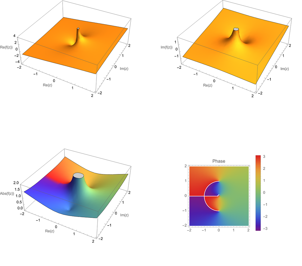
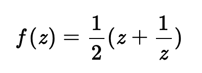
f[z_]:=(1/2)*(z+1/z);

plotComplexFunction[f]
https://github.com/dreamchef/complex-functions-visualization

https://github.com/dreamchef/complex-functions-visualization

I wrote the above Mathematica code to produce a grid of plots showing the function in both ways just described. On the top, the imaginary and real parts of the function

are shown, and on the bottom, and the magnitude, and the phase shown in color:

After playing around with a few functions using this code and convincing myself they made sense, I was interested in getting the same functionality in Python, to connect it to my other mathematical programming projects.

Python, PyPlot and complex-plotting-tools

I found an excellent project on GitHub (https://github.com/artmenlope/complex-plotting-tools) which I decided to use as a starting point, and potentially contribute to in the future. The repo provided a very easy interface for plotting complex-valued functions in a variety of ways. Thanks https://github.com/artmenlope! For example, after importing numpy, matplotlib, and the repo’s cplotting_tools module defining the function and calling cplt.complex_plot3D(x,y,f,log_mode=False) produces the following:

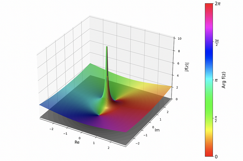
These are all for the same f(z) as above. To view the side-by-side imaginary and real parts of the function, use cplot.plot_re_im(x,y,f,camp="twilight",contour=False,alpha=0.9:

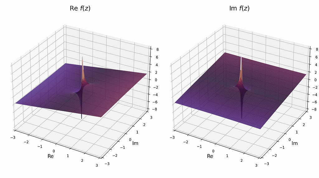
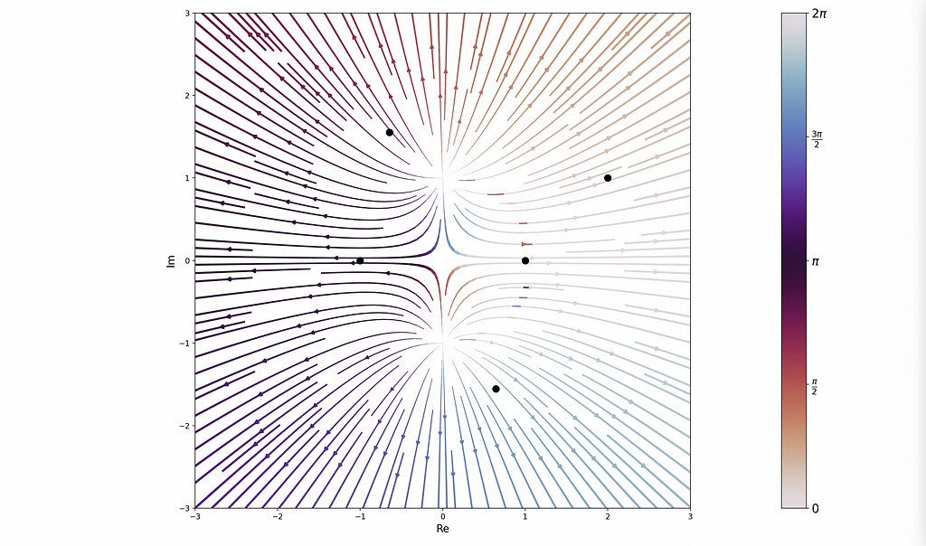
Additionally, the library provides other cool ways to study functions, including a stream plot:

Future Direction

The library shows a lot of promise and is relatively easy to use! It does require a pts variable to be defined that encodes the poles and zeros of the given function. Wolfram does not require this because it computes the locations of these points under the hood. It would save a lot of effort for the user if complex-plotting-tools had this functionality as well. I plan to implement this is into the module in the near future.

In the meantime, have fun plotting with Wolfram and Python, and send any questions or development ideas my way.

Cheers!

Dani

Unless otherwise noted, all images were created by the author.

Visualizing Complex-Valued Functions Using Python and Mathematica was originally published in Towards Data Science on Medium, where people are continuing the conversation by highlighting and responding to this story.

Visualizing Complex-Valued Functions in Python and Mathematica

Unlocking visual insights into a difficult but powerful branch of math

Today I was pouring through Complex Variables and Analytic Functions by the esteemed Fornberg and Piret, trying my best to wrap my mind around how complex-valued functions behave. Mentally vizualization such functions is extra difficult since they take a real and an imaginary input, and outputs two components as well. Therefore, a single 3-D plot is not sufficient to see how the function behaves. Rather, we have to split such a visualization into separate plots of the imaginary and real parts, or alternatively by magnitude and argument, or angle.

I wanted to be able to play around with any function I could think of, drag and zoom around its plots, and explore it in visual detail to understand how it resulted from the equation. For such a task, Wolfram Mathematica is an excellent starting tool.

Wolfram Language

plotComplexFunction[f_]:=Module[{z,rePlot,imPlot,magPlot,phasePlot},z=x+I y;

rePlot = Plot3D[Re[f[z]],{x,-2,2},{y,-2,2},AxesLabel->{"Re(z)","Im(z)","Re(f(z))"},Mesh->None];

imPlot = Plot3D[Im[f[z]],{x,-2,2},{y,-2,2},
 AxesLabel->{"Re(z)","Im(z)","Im(f(z))"},
 Mesh->None];

magPlot = Plot3D[Abs[f[z]], {x, -2, 2}, {y, -2, 2}, 
 AxesLabel -> {"Re(z)", "Im(z)", "Abs(f(z))"}, 
 Mesh -> None, 
 ColorFunction -> Function[{x, y, z}, ColorData["Rainbow"][Rescale[Arg[x + I y], {-Pi, Pi}]]], 
 ColorFunctionScaling -> False];
 
phasePlot=DensityPlot[Arg[f[z]],{x,-2,2},{y,-2,2},
 ColorFunction->"Rainbow",
 PlotLegends->Automatic,
 AxesLabel->{"Re(z)","Im(z)"},
 PlotLabel->"Phase"];

GraphicsGrid[{{rePlot,imPlot},{magPlot,phasePlot}},ImageSize->800]];

f[z_]:=(1/2)*(z+1/z);

plotComplexFunction[f]
https://github.com/dreamchef/complex-functions-visualization

https://github.com/dreamchef/complex-functions-visualization

I wrote the above Mathematica code to produce a grid of plots showing the function in both ways just described. On the top, the imaginary and real parts of the function

are shown, and on the bottom, and the magnitude, and the phase shown in color:

After playing around with a few functions using this code and convincing myself they made sense, I was interested in getting the same functionality in Python, to connect it to my other mathematical programming projects.

Python, PyPlot and complex-plotting-tools

I found an excellent project on GitHub (https://github.com/artmenlope/complex-plotting-tools) which I decided to use as a starting point, and potentially contribute to in the future. The repo provided a very easy interface for plotting complex-valued functions in a variety of ways. Thanks https://github.com/artmenlope! For example, after importing numpy, matplotlib, and the repo’s cplotting_tools module defining the function and calling cplt.complex_plot3D(x,y,f,log_mode=False) produces the following:

These are all for the same f(z) as above. To view the side-by-side imaginary and real parts of the function, use cplot.plot_re_im(x,y,f,camp="twilight",contour=False,alpha=0.9:

Additionally, the library provides other cool ways to study functions, including a stream plot:

Future Direction

The library shows a lot of promise and is relatively easy to use! It does require a pts variable to be defined that encodes the poles and zeros of the given function. Wolfram does not require this because it computes the locations of these points under the hood. It would save a lot of effort for the user if complex-plotting-tools had this functionality as well. I plan to implement this is into the module in the near future.

In the meantime, have fun plotting with Wolfram and Python, and send any questions or development ideas my way.

Cheers!

Dani

Unless otherwise noted, all images were created by the author.

Visualizing Complex-Valued Functions Using Python and Mathematica was originally published in Towards Data Science on Medium, where people are continuing the conversation by highlighting and responding to this story.

FOLLOW US ON GOOGLE NEWS

Read original article here