
Visualizing Gradient Descent Parameters in Torch
Prying behind the interface to see the effects of SGD parameters on your model training
Behind the simple interfaces of modern machine learning frameworks lie large amounts of complexity. With so many dials and knobs exposed to us, we could easily fall into cargo cult programming if we don’t understand what’s going on underneath. Consider the many parameters of Torch’s stochastic gradient descent (SGD) optimizer:
def torch.optim.SGD(
  params, lr=0.001, momentum=0, dampening=0,
  weight_decay=0, nesterov=False, *, maximize=False,
  foreach=None, differentiable=False):
  # Implements stochastic gradient descent (optionally with momentum).
  # ...
Besides the familiar learning rate lr and momentum parameters, there are several other that have stark effects on neural network training. In this article we’ll visualize the effects of these parameters on a simple ML objective with a variety of loss functions.
Toy Problem
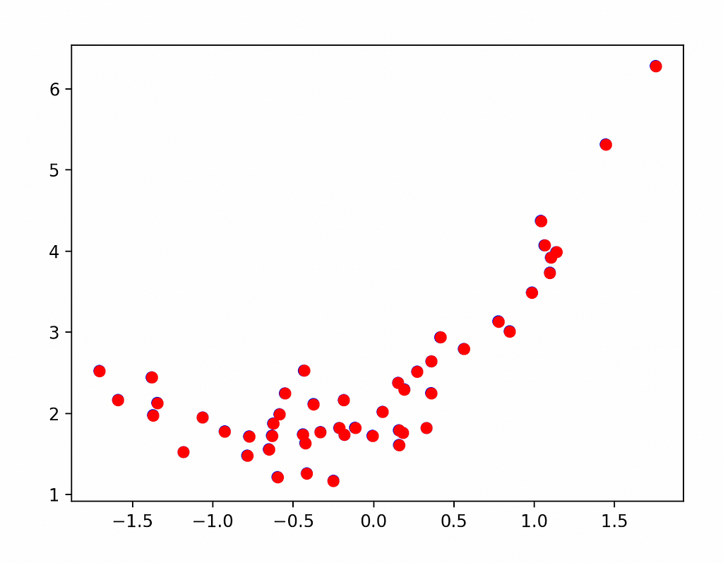
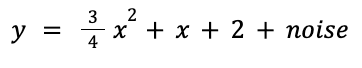
To start we construct a toy problem of performing linear regression over a set of points. To make it interesting we’re going to use a quadratic function plus noise so that the neural network will have to make trade-offs—and we’ll also get to observe more of the impact of the loss functions:
We start off just using numpy and matplotlib to visualization our data—no torch required yet:
import numpy as np
import matplotlib.pyplot as plt

np.random.seed(20240215)
n = 50
x = np.array(np.random.randn(n), dtype=np.float32)
y = np.array(
  0.75 * x**2 + 1.0 * x + 2.0 + 0.3 * np.random.randn(n),
  dtype=np.float32)

plt.scatter(x, y, facecolors='none', edgecolors='b')
plt.scatter(x, y, c='r')
plt.show()
Next we’ll break out the torch and introduce a simple training loop for a single-neuron network. To get consistent results when we vary the loss function, we’ll start our training from the same set of parameters each time with the neuron’s first “guess” being the equation y = 6*x — 3 (which we effect via the neuron’s weight and bias parameters):
import torch

model = torch.nn.Linear(1, 1)
model.weight.data.fill_(6.0)
model.bias.data.fill_(-3.0)

loss_fn = torch.nn.MSELoss()
learning_rate = 0.1
epochs = 100
optimizer = torch.optim.SGD(model.parameters(), lr=learning_rate)

for epoch in range(epochs):
  inputs = torch.from_numpy(x).requires_grad_().reshape(-1, 1)
  labels = torch.from_numpy(y).reshape(-1, 1)

  optimizer.zero_grad()
  outputs = model(inputs)
  loss = loss_fn(outputs, labels)
  loss.backward()
  optimizer.step()
  print('epoch {}, loss {}'.format(epoch, loss.item()))
Running this gives us text output that shows us the loss is decreasing, eventually down to a minimum, as expected:
epoch 0, loss 53.078269958496094
epoch 1, loss 34.7295036315918
epoch 2, loss 22.891206741333008
epoch 3, loss 15.226042747497559
epoch 4, loss 10.242652893066406
epoch 5, loss 6.987757682800293
epoch 6, loss 4.85075569152832
epoch 7, loss 3.4395809173583984
epoch 8, loss 2.501774787902832
epoch 9, loss 1.8742430210113525
...
epoch 97, loss 0.4994412660598755
epoch 98, loss 0.4994412362575531
epoch 99, loss 0.4994412660598755
To visualize our fit, we take the learned bias and weight out of our neuron and plot the fit against the points:
weight = model.weight.item()
bias = model.bias.item()
plt.scatter(x, y, facecolors='none', edgecolors='b')
plt.plot(
  [x.min(), x.max()],
  [weight * x.min() + bias, weight * x.max() + bias],
  c='r')
plt.show()

Visualizing the Loss Function
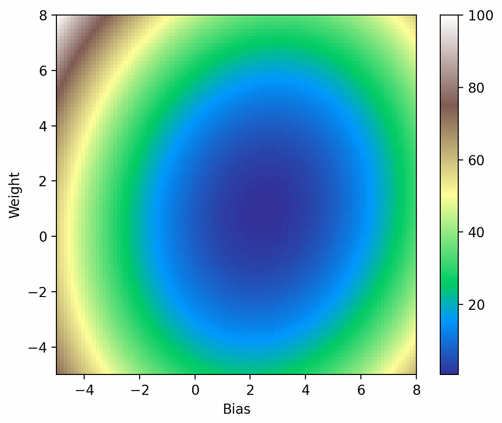
The above seems a reasonable fit, but so far everything has been handled by high-level Torch functions like optimizer.zero_grad(), loss.backward(), and optimizer.step(). To understand where we’re going next, we’ll need to visualize the journey our model is taking through the loss function. To visualize the loss, we’ll sample it in a grid of 101-by-101 points, then plot it using imshow:
def get_loss_map(loss_fn, x, y):
  """Maps the loss function on a 100-by-100 grid between (-5, -5) and (8, 8)."""
  losses = [[0.0] * 101 for _ in range(101)]
  x = torch.from_numpy(x)
  y = torch.from_numpy(y)
  for wi in range(101):
    for wb in range(101):
      w = -5.0 + 13.0 * wi / 100.0
      b = -5.0 + 13.0 * wb / 100.0
      ywb = x * w + b
      losses[wi][wb] = loss_fn(ywb, y).item()

  return list(reversed(losses))  # Because y will be reversed.

import pylab

loss_fn = torch.nn.MSELoss()
losses = get_loss_map(loss_fn, x, y)
cm = pylab.get_cmap('terrain')

fig, ax = plt.subplots()
plt.xlabel('Bias')
plt.ylabel('Weight')
i = ax.imshow(losses, cmap=cm, interpolation='nearest', extent=[-5, 8, -5, 8])
fig.colorbar(i)
plt.show()
Now we can capture the model parameters while running gradient descent to show us how the optimizer is performing:
model = torch.nn.Linear(1, 1)
...
models = [[model.weight.item(), model.bias.item()]]
for epoch in range(epochs):
  ...
  print('epoch {}, loss {}'.format(epoch, loss.item()))
  models.append([model.weight.item(), model.bias.item()])

# Plot model parameters against the loss map.
cm = pylab.get_cmap('terrain')
fig, ax = plt.subplots()
plt.xlabel('Bias')
plt.ylabel('Weight')
i = ax.imshow(losses, cmap=cm, interpolation='nearest', extent=[-5, 8, -5, 8])

model_weights, model_biases = zip(*models)
ax.scatter(model_biases, model_weights, c='r', marker='+')
ax.plot(model_biases, model_weights, c='r')

fig.colorbar(i)
plt.show()
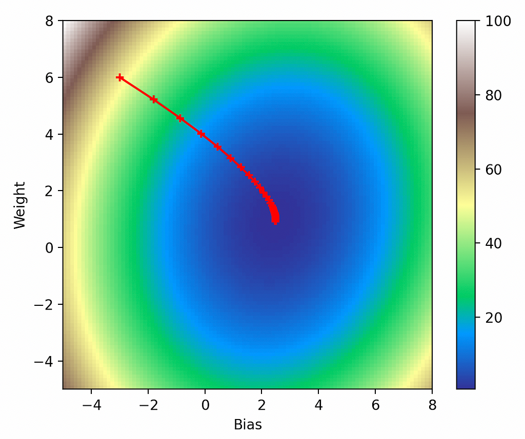
From inspection this looks exactly as it should: the model starts off at our force-initialized parameters of (-3, 6), it takes progressively smaller steps in the direction of the gradient, and it eventually bottoms-out in the global minimum.
Visualizing the Other Parameters
Loss Function
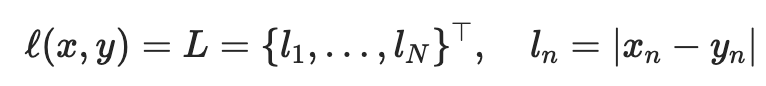
Now we’ll start examining the effects of the other parameters on gradient descent. First is the loss function, for which we used the standard L2 loss:

But there are several other loss functions we could use:
We wrap everything we’ve done so far in a loop to try out all the loss functions and plot them together:
def multi_plot(lr=0.1, epochs=100, momentum=0, weight_decay=0, dampening=0, nesterov=False):
fig, ((ax1, ax2), (ax3, ax4)) = plt.subplots(2, 2)
for loss_fn, title, ax in [
(torch.nn.MSELoss(), 'MSELoss', ax1),
(torch.nn.L1Loss(), 'L1Loss', ax2),
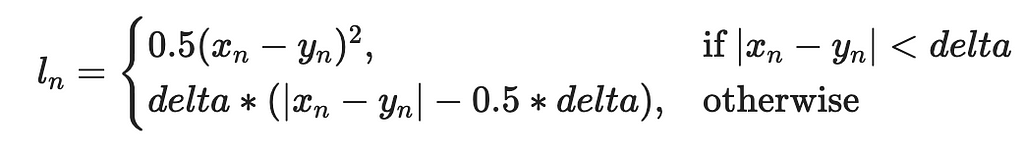
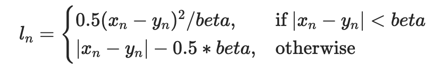
(torch.nn.HuberLoss(), 'HuberLoss', ax3),
(torch.nn.SmoothL1Loss(), 'SmoothL1Loss', ax4),
]:
losses = get_loss_map(loss_fn, x, y)
model, models = learn(
loss_fn, x, y, lr=lr, epochs=epochs, momentum=momentum,
weight_decay=weight_decay, dampening=dampening, nesterov=nesterov)
cm = pylab.get_cmap('terrain')
i = ax.imshow(losses, cmap=cm, interpolation='nearest', extent=[-5, 8, -5, 8])
ax.title.set_text(title)
loss_w, loss_b = zip(*models)
ax.scatter(loss_b, loss_w, c='r', marker='+')
ax.plot(loss_b, loss_w, c='r')
plt.show()
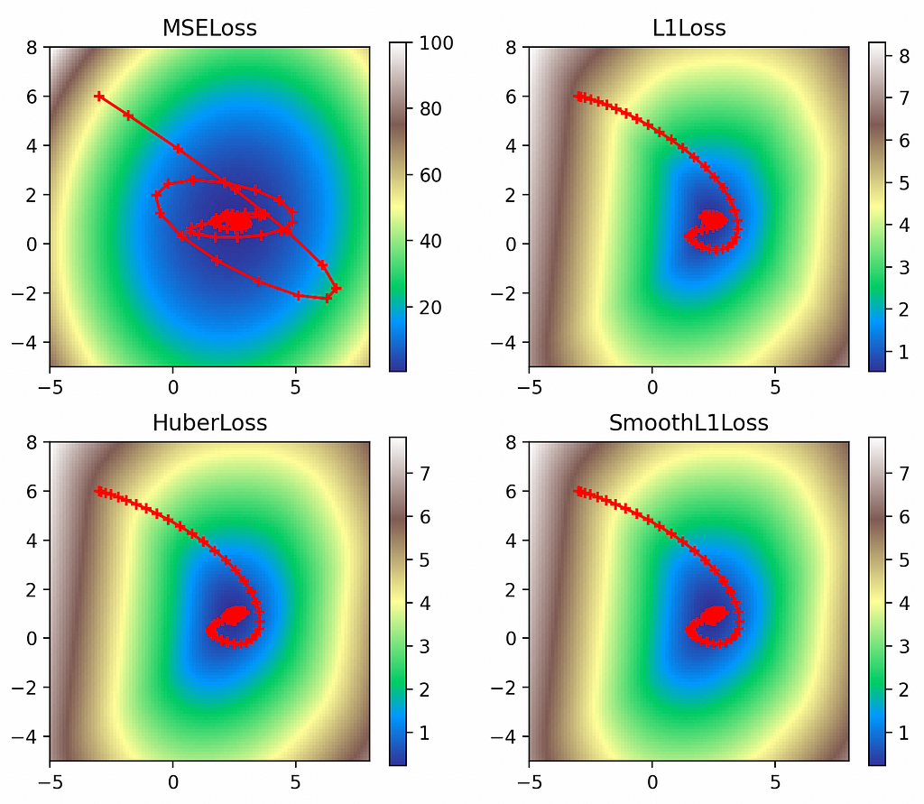
multi_plot(lr=0.1, epochs=100)

Here we can see the interesting contours of the non-L2 loss functions. While the L2 loss function is smooth and exhibits large values up to 100, the other loss functions have much smaller values as they reflect only the absolute errors. But the L2 loss’s steeper gradient means the optimizer makes a quicker approach to the global minimum, as evidenced by the greater spacing between its early points. Meanwhile the L1 losses all display much more gradual approaches to their minima.
Momentum
The next most interesting parameter is the momentum, which dictates how much of the last step’s gradient to add in to the current gradient update going froward. Normally very small values of momentum are sufficient, but for the sake of visualization we’re going to set it to the crazy value of 0.9—kids, do NOT try this at home:
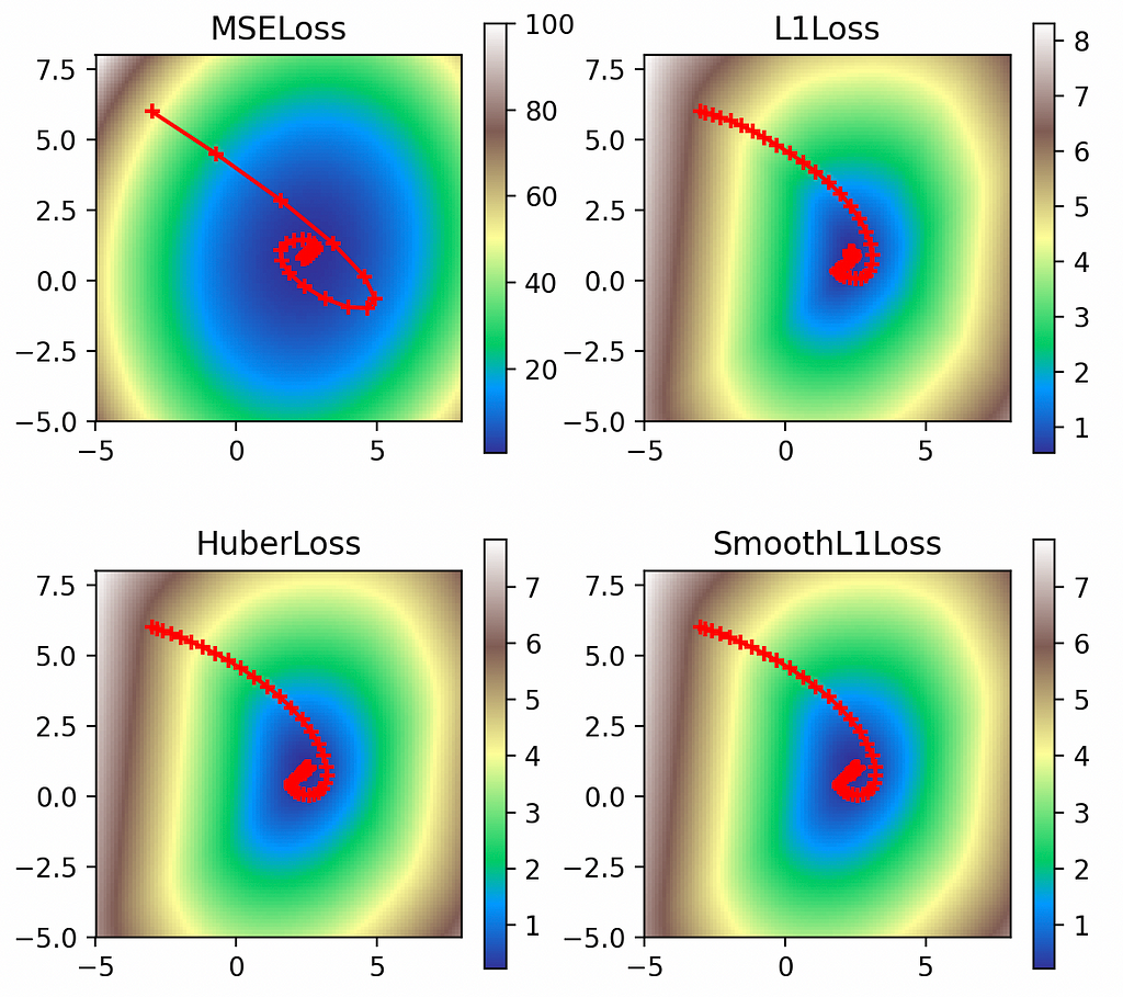
multi_plot(lr=0.1, epochs=100, momentum=0.9)
Thanks to the outrageous momentum value, we can clearly see its effect on the optimizer: it overshoots the global minimum and has to swerve sloppily back around. This effect is most pronounced in the L2 loss, whose steep gradients carry it clean over the minimum and bring it very close to diverging.
Nesterov Momentum
Nesterov momentum is an interesting tweak on momentum. Normal momentum adds in some of the gradient from the last step to the gradient for the current step, giving us the scenario in figure 7(a) below. But if we already know where the gradient from the last step is going to carry us, then Nesterov momentum instead calculates the current gradient by looking ahead to where that will be, giving us the scenario in figure 7(b) below:
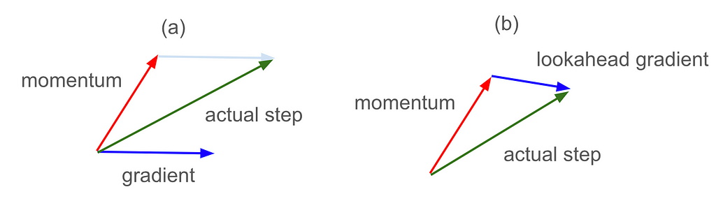
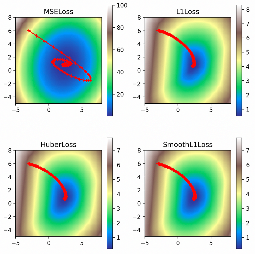
multi_plot(lr=0.1, epochs=100, momentum=0.9, nesterov=True)
When viewed graphically, we can see that Nesterov momentum has cut down the overshooting we observed with plain momentum. Especially in the L2 case, since our momentum carried us clear over the global minimum, using Nesterov to lookahead where we were going to land allowed us to mix in countervailing gradients from the opposite side of the objective function, in effect course-correcting earlier.
Weight Decay
Next weight decay adds a regularizing L2 penalty on the values of the parameters (the weight and bias of our linear network):
multi_plot(lr=0.1, epochs=100, momentum=0.9, nesterov=True, weight_decay=2.0)
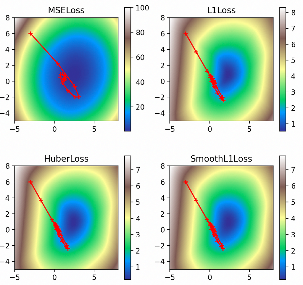
In all cases, the regularizing factor has pulled the solutions away from their rightful global minima and closer to the origin (0, 0). The effect is least pronounced with the L2 loss, however, since the loss values are large enough to offset the L2 penalties on the weights.
Dampening
Finally we have dampening, which discounts the momentum by the dampening factor. Using a dampening factor of 0.8 we see how it effectively moderates the momentum path through the loss function.
multi_plot(lr=0.1, epochs=100, momentum=0.9, dampening=0.8)
Unless otherwise noted, all images are by the author.
References
- https://pytorch.org/docs/stable/generated/torch.nn.MSELoss.html
- https://pytorch.org/docs/stable/generated/torch.nn.L1Loss.html
- https://pytorch.org/docs/stable/generated/torch.nn.HuberLoss.html
- https://pytorch.org/docs/stable/generated/torch.nn.SmoothL1Loss.html
- https://pytorch.org/docs/stable/generated/torch.optim.SGD.html
See Also
- https://towardsdatascience.com/extending-context-length-in-large-language-models-74e59201b51f
- Code available at: https://github.com/pbaumstarck/scaling-invention/blob/main/code/torch_loss.py
- https://github.com/tomgoldstein/loss-landscape
- https://neptune.ai/blog/pytorch-loss-functions
Visualizing Gradient Descent Parameters in Torch was originally published in Towards Data Science on Medium, where people are continuing the conversation by highlighting and responding to this story.
Prying behind the interface to see the effects of SGD parameters on your model training
Behind the simple interfaces of modern machine learning frameworks lie large amounts of complexity. With so many dials and knobs exposed to us, we could easily fall into cargo cult programming if we don’t understand what’s going on underneath. Consider the many parameters of Torch’s stochastic gradient descent (SGD) optimizer:
def torch.optim.SGD(
  params, lr=0.001, momentum=0, dampening=0,
  weight_decay=0, nesterov=False, *, maximize=False,
  foreach=None, differentiable=False):
  # Implements stochastic gradient descent (optionally with momentum).
  # ...
Besides the familiar learning rate lr and momentum parameters, there are several other that have stark effects on neural network training. In this article we’ll visualize the effects of these parameters on a simple ML objective with a variety of loss functions.
Toy Problem
To start we construct a toy problem of performing linear regression over a set of points. To make it interesting we’re going to use a quadratic function plus noise so that the neural network will have to make trade-offs—and we’ll also get to observe more of the impact of the loss functions:
We start off just using numpy and matplotlib to visualization our data—no torch required yet:
import numpy as np
import matplotlib.pyplot as plt

np.random.seed(20240215)
n = 50
x = np.array(np.random.randn(n), dtype=np.float32)
y = np.array(
  0.75 * x**2 + 1.0 * x + 2.0 + 0.3 * np.random.randn(n),
  dtype=np.float32)

plt.scatter(x, y, facecolors='none', edgecolors='b')
plt.scatter(x, y, c='r')
plt.show()
Next we’ll break out the torch and introduce a simple training loop for a single-neuron network. To get consistent results when we vary the loss function, we’ll start our training from the same set of parameters each time with the neuron’s first “guess” being the equation y = 6*x — 3 (which we effect via the neuron’s weight and bias parameters):
import torch

model = torch.nn.Linear(1, 1)
model.weight.data.fill_(6.0)
model.bias.data.fill_(-3.0)

loss_fn = torch.nn.MSELoss()
learning_rate = 0.1
epochs = 100
optimizer = torch.optim.SGD(model.parameters(), lr=learning_rate)

for epoch in range(epochs):
  inputs = torch.from_numpy(x).requires_grad_().reshape(-1, 1)
  labels = torch.from_numpy(y).reshape(-1, 1)

  optimizer.zero_grad()
  outputs = model(inputs)
  loss = loss_fn(outputs, labels)
  loss.backward()
  optimizer.step()
  print('epoch {}, loss {}'.format(epoch, loss.item()))
Running this gives us text output that shows us the loss is decreasing, eventually down to a minimum, as expected:
epoch 0, loss 53.078269958496094
epoch 1, loss 34.7295036315918
epoch 2, loss 22.891206741333008
epoch 3, loss 15.226042747497559
epoch 4, loss 10.242652893066406
epoch 5, loss 6.987757682800293
epoch 6, loss 4.85075569152832
epoch 7, loss 3.4395809173583984
epoch 8, loss 2.501774787902832
epoch 9, loss 1.8742430210113525
...
epoch 97, loss 0.4994412660598755
epoch 98, loss 0.4994412362575531
epoch 99, loss 0.4994412660598755
To visualize our fit, we take the learned bias and weight out of our neuron and plot the fit against the points:
weight = model.weight.item()
bias = model.bias.item()
plt.scatter(x, y, facecolors='none', edgecolors='b')
plt.plot(
  [x.min(), x.max()],
  [weight * x.min() + bias, weight * x.max() + bias],
  c='r')
plt.show()
Visualizing the Loss Function
The above seems a reasonable fit, but so far everything has been handled by high-level Torch functions like optimizer.zero_grad(), loss.backward(), and optimizer.step(). To understand where we’re going next, we’ll need to visualize the journey our model is taking through the loss function. To visualize the loss, we’ll sample it in a grid of 101-by-101 points, then plot it using imshow:
def get_loss_map(loss_fn, x, y):
  """Maps the loss function on a 100-by-100 grid between (-5, -5) and (8, 8)."""
  losses = [[0.0] * 101 for _ in range(101)]
  x = torch.from_numpy(x)
  y = torch.from_numpy(y)
  for wi in range(101):
    for wb in range(101):
      w = -5.0 + 13.0 * wi / 100.0
      b = -5.0 + 13.0 * wb / 100.0
      ywb = x * w + b
      losses[wi][wb] = loss_fn(ywb, y).item()

  return list(reversed(losses))  # Because y will be reversed.

import pylab

loss_fn = torch.nn.MSELoss()
losses = get_loss_map(loss_fn, x, y)
cm = pylab.get_cmap('terrain')

fig, ax = plt.subplots()
plt.xlabel('Bias')
plt.ylabel('Weight')
i = ax.imshow(losses, cmap=cm, interpolation='nearest', extent=[-5, 8, -5, 8])
fig.colorbar(i)
plt.show()
Now we can capture the model parameters while running gradient descent to show us how the optimizer is performing:
model = torch.nn.Linear(1, 1)
...
models = [[model.weight.item(), model.bias.item()]]
for epoch in range(epochs):
  ...
  print('epoch {}, loss {}'.format(epoch, loss.item()))
  models.append([model.weight.item(), model.bias.item()])

# Plot model parameters against the loss map.
cm = pylab.get_cmap('terrain')
fig, ax = plt.subplots()
plt.xlabel('Bias')
plt.ylabel('Weight')
i = ax.imshow(losses, cmap=cm, interpolation='nearest', extent=[-5, 8, -5, 8])

model_weights, model_biases = zip(*models)
ax.scatter(model_biases, model_weights, c='r', marker='+')
ax.plot(model_biases, model_weights, c='r')

fig.colorbar(i)
plt.show()
From inspection this looks exactly as it should: the model starts off at our force-initialized parameters of (-3, 6), it takes progressively smaller steps in the direction of the gradient, and it eventually bottoms-out in the global minimum.
Visualizing the Other Parameters
Loss Function
Now we’ll start examining the effects of the other parameters on gradient descent. First is the loss function, for which we used the standard L2 loss:
But there are several other loss functions we could use:
We wrap everything we’ve done so far in a loop to try out all the loss functions and plot them together:
def multi_plot(lr=0.1, epochs=100, momentum=0, weight_decay=0, dampening=0, nesterov=False):
  fig, ((ax1, ax2), (ax3, ax4)) = plt.subplots(2, 2)
  for loss_fn, title, ax in [
    (torch.nn.MSELoss(), 'MSELoss', ax1),
    (torch.nn.L1Loss(), 'L1Loss', ax2),
    (torch.nn.HuberLoss(), 'HuberLoss', ax3),
    (torch.nn.SmoothL1Loss(), 'SmoothL1Loss', ax4),
  ]:
    losses = get_loss_map(loss_fn, x, y)
    model, models = learn(
      loss_fn, x, y, lr=lr, epochs=epochs, momentum=momentum,
      weight_decay=weight_decay, dampening=dampening, nesterov=nesterov)

    cm = pylab.get_cmap('terrain')
    i = ax.imshow(losses, cmap=cm, interpolation='nearest', extent=[-5, 8, -5, 8])
    ax.title.set_text(title)
    loss_w, loss_b = zip(*models)
    ax.scatter(loss_b, loss_w, c='r', marker='+')
    ax.plot(loss_b, loss_w, c='r')

  plt.show()

multi_plot(lr=0.1, epochs=100)
Here we can see the interesting contours of the non-L2 loss functions. While the L2 loss function is smooth and exhibits large values up to 100, the other loss functions have much smaller values as they reflect only the absolute errors. But the L2 loss’s steeper gradient means the optimizer makes a quicker approach to the global minimum, as evidenced by the greater spacing between its early points. Meanwhile the L1 losses all display much more gradual approaches to their minima.
Momentum
The next most interesting parameter is the momentum, which dictates how much of the last step’s gradient to add in to the current gradient update going froward. Normally very small values of momentum are sufficient, but for the sake of visualization we’re going to set it to the crazy value of 0.9—kids, do NOT try this at home:
multi_plot(lr=0.1, epochs=100, momentum=0.9)
Thanks to the outrageous momentum value, we can clearly see its effect on the optimizer: it overshoots the global minimum and has to swerve sloppily back around. This effect is most pronounced in the L2 loss, whose steep gradients carry it clean over the minimum and bring it very close to diverging.
Nesterov Momentum
Nesterov momentum is an interesting tweak on momentum. Normal momentum adds in some of the gradient from the last step to the gradient for the current step, giving us the scenario in figure 7(a) below. But if we already know where the gradient from the last step is going to carry us, then Nesterov momentum instead calculates the current gradient by looking ahead to where that will be, giving us the scenario in figure 7(b) below:
multi_plot(lr=0.1, epochs=100, momentum=0.9, nesterov=True)
When viewed graphically, we can see that Nesterov momentum has cut down the overshooting we observed with plain momentum. Especially in the L2 case, since our momentum carried us clear over the global minimum, using Nesterov to lookahead where we were going to land allowed us to mix in countervailing gradients from the opposite side of the objective function, in effect course-correcting earlier.
Weight Decay
Next weight decay adds a regularizing L2 penalty on the values of the parameters (the weight and bias of our linear network):
multi_plot(lr=0.1, epochs=100, momentum=0.9, nesterov=True, weight_decay=2.0)
In all cases, the regularizing factor has pulled the solutions away from their rightful global minima and closer to the origin (0, 0). The effect is least pronounced with the L2 loss, however, since the loss values are large enough to offset the L2 penalties on the weights.
Dampening
Finally we have dampening, which discounts the momentum by the dampening factor. Using a dampening factor of 0.8 we see how it effectively moderates the momentum path through the loss function.
multi_plot(lr=0.1, epochs=100, momentum=0.9, dampening=0.8)
Unless otherwise noted, all images are by the author.
References
- https://pytorch.org/docs/stable/generated/torch.nn.MSELoss.html
- https://pytorch.org/docs/stable/generated/torch.nn.L1Loss.html
- https://pytorch.org/docs/stable/generated/torch.nn.HuberLoss.html
- https://pytorch.org/docs/stable/generated/torch.nn.SmoothL1Loss.html
- https://pytorch.org/docs/stable/generated/torch.optim.SGD.html
See Also
- https://towardsdatascience.com/extending-context-length-in-large-language-models-74e59201b51f
- Code available at: https://github.com/pbaumstarck/scaling-invention/blob/main/code/torch_loss.py
- https://github.com/tomgoldstein/loss-landscape
- https://neptune.ai/blog/pytorch-loss-functions
Visualizing Gradient Descent Parameters in Torch was originally published in Towards Data Science on Medium, where people are continuing the conversation by highlighting and responding to this story.
Denial of responsibility! Techno Blender is an automatic aggregator of the all world’s media. In each content, the hyperlink to the primary source is specified. All trademarks belong to their rightful owners, all materials to their authors. If you are the owner of the content and do not want us to publish your materials, please contact us by email – [email protected]. The content will be deleted within 24 hours.