What’s The Story With HNSW?

Exploring the path to fast nearest neighbour search with Hierarchical Navigable Small Worlds

Hierarchical Navigable Small World (HNSW) has become popular as one of the best performing approaches for approximate nearest neighbour search. HNSW is a little complex though, and descriptions often lack a complete and intuitive explanation. This post takes a journey through the history of the HNSW idea to help explain what “hierarchical navigable small world” actually means and why it’s effective.

Contents

• Approximate Nearest Neighbour Search
• Small Worlds
• Navigable Small Worlds
• Hierarchical Navigable Small Worlds
• Summary
• Appendix
  – Improved search
  – HNSW search & insertion
  – Improved insertion
• References

Approximate Nearest Neighbour Search

A common application of machine learning is nearest neighbour search, which means finding the most similar items* to a target — for example, to recommend items that are similar to a user’s preferences, or to search for items that are similar to a user’s search query.

The simple method is to calculate the similarity of every item to the target and return the closest ones. However, if there are a large number of items (maybe millions), this will be slow.

Instead, we can use a structure called an index to make things much faster.

There is a trade-off, however. Unlike the simple method, indexes only give approximate results: we may not retrieve all of the nearest neighbours (i.e. recall may be less than 100%).

There are several different types of index (e.g. locality sensitive hashing; inverted file index), but HNSW has proven particularly effective on various datasets, achieving high speeds while keeping high recall.

*Typically, items are represented as embeddings, which are vectors produced by a machine learning model; the similarity between items corresponds to the distance between the embeddings. This post will usually talk of vectors and distances, though in general HNSW can handle any kind of items with some measure of similarity.

Small Worlds

Small worlds were famously studied in Stanley Milgram’s small-world experiment [1].

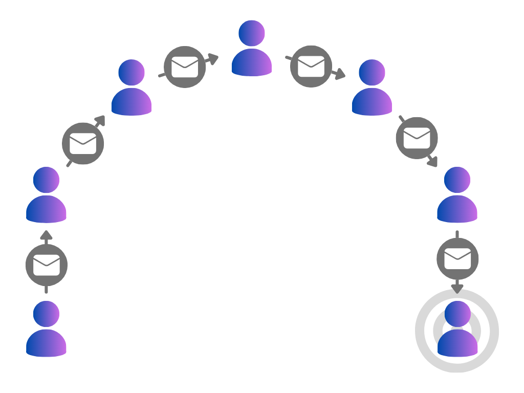
Participants were given a letter containing the address and other basic details of a randomly chosen target individual, along with the experiment’s instructions. In the unlikely event that they personally knew the target, they were instructed to send them the letter; otherwise, they were told to think of someone they knew who was more likely to know the target, and send the letter on to them.

The surprising conclusion was that the letters were typically only sent around six times before reaching the target, demonstrating the famous idea of “six degrees of separation” — any two people can usually be connected by a small chain of friends.

In the mathematical field of graph theory, a graph is a set of points, some of which are connected. We can think of a social network as a graph, with people as points and friendships as connections. The small-world experiment found that most pairs of points in this graph are connected by short paths that have a small number of steps. (This is described technically as the graph having a low diameter.)

Having short paths is not that surprising in itself: most graphs have this property, including graphs created by just connecting random pairs of points. But social networks are not connected randomly, they are highly local: friends tend to live close to each other, and if you know two people, it’s quite likely they know each other too. (This is described technically as the graph having a high clustering coefficient.) The surprising thing about the small-world experiment is that two distant points are only separated by a short path despite connections typically being short-range.

In cases like these when a graph has lots of local connections, but also has short paths, we say the graph is a small world.

Another good example of a small world is the global airport network. Airports in the same region are highly connected to one another, but it’s possible to make a long journey in only a few stops by making use of major hub airports. For example, a journey from Manchester, UK to Osaka, Japan typically starts with a local flight from Manchester to London, then a long distance flight from London to Tokyo, and finally another local flight from Tokyo to Osaka. Long-range hubs are a common way of achieving the small world property.

A final interesting example of graphs with the small world property is biological neural networks such as the human brain.

Navigable Small Worlds

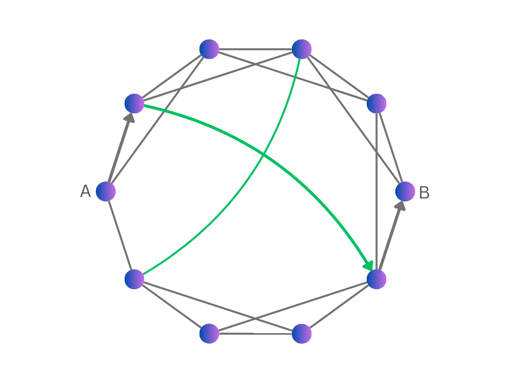
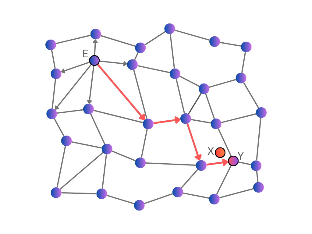
In small world graphs, we can quickly reach a target in a few steps. This suggests a promising idea for nearest neighbour search: perhaps if we create connections between our vectors in such a way that it forms a small world graph, we can quickly find the vectors near a target by starting from an arbitrary “entry point” vector and then navigating through the graph towards the target.

This possibility was explored by Kleinberg [2]. He noted that the existence of short paths wasn’t the only interesting thing about Miller’s experiment: it was also surprising that people were able to find these short paths, without using any global knowledge about the graph. Rather, the people were following a simple greedy algorithm. At each step, they examined each of their immediate connections, and sent it to the one they thought was closest to the target. We can use a similar algorithm to search a graph that connects vectors.

Kleinberg wanted to know whether this greedy algorithm would always find a short path. He ran simple simulations of small worlds in which all of the points were connected to their immediate neighbours, with additional longer connections created between random points. He discovered that the greedy algorithm would only find a short path in specific conditions, depending on the lengths of the long-range connections.

If the long-range connections were too long (as was the case when they connected pairs of points in completely random locations), the greedy algorithm could follow a long-range connection to quickly reach the rough area of the target, but after that the long-range connections were of no use, and the path had to step through the local connections to get closer. On the other hand, if the long-range connections were too short, it would simply take too many steps to reach the area of the target.

If, however, the lengths of the long-range connections were just right (to be precise, if they were uniformly distributed, so that all lengths were equally likely), the greedy algorithm would typically reach the neighbourhood of the target in an especially small number of steps (to be more specific, a number proportional to log(n), where n is the number of points in the graph).

In cases like this where the greedy algorithm can find the target in a small number of steps, we say the small world is a navigable small world (NSW).

An NSW sounds like an ideal index for our vectors, but for vectors in a complex, high-dimensional space, it’s not clear how to actually build one. Fortunately, Malkov et al. [3] discovered a method: we insert one randomly chosen vector at a time to the graph, and connect it to a small number m of nearest neighbours that were already inserted.

This method is remarkably simple and requires no global understanding of how the vectors are distributed in space. It’s also very efficient, as we can use the graph built so far to perform the nearest neighbour search for inserting each vector.

Experiments confirmed that this method produces an NSW. Because the vectors inserted early on are randomly chosen, they tend to be quite far apart. They therefore form the long-range connections needed for a small world. It’s not so obvious why the small world is navigable, but as we insert more vectors, the connections will get gradually shorter, so it’s plausible that the distribution of connection lengths will be fairly even, as required.

Hierarchical Navigable Small Worlds

Navigable small worlds can work well for approximate nearest neighbours search, but further analysis revealed areas for improvement, leading Markov et al. [4] to propose HNSW.

A typical path through an NSW from the entry point towards the target went through two phases: a “zoom-out” phase, in which connection lengths increase from short to long, and a “zoom-in” phase, in which the reverse happens.

The first simple improvement is to use a long-range hub (such as the first inserted vector) as the entry point. This way, we can skip the zoom-out phase and go straight to the zoom-in phase.

Secondly, although the search paths were short (with a number of steps proportional to log(n)), the whole search procedure wasn’t so fast. At each vector along the path, the greedy algorithm must examine each of the connected vectors, calculating their distance to the target in order to choose the closest one. While most of the locally connected vectors had only a few connections, most long-range hubs had many connections (again, a number proportional to log(n)); this makes sense as these vectors were usually inserted early on in the building process and had many opportunities to connect to other vectors. As a result, the total number of calculations during a search was quite large (proportional to log(n)²).

To improve this, we need to limit the number of connections checked at each hub. This leads to the main idea of HNSW: explicitly distinguishing between short-range and long-range connections. In the initial stage of a search, we will only consider the long-range connections between hubs. Once the greedy search has found a hub near the target, we then switch to using the short-range connections.

As the number of hubs is relatively small, they should have few connections to check. We can also explicitly impose a maximum number of long-range and short-range connections of each vector when we build the index. This results in a fast search time (proportional to log(n)).

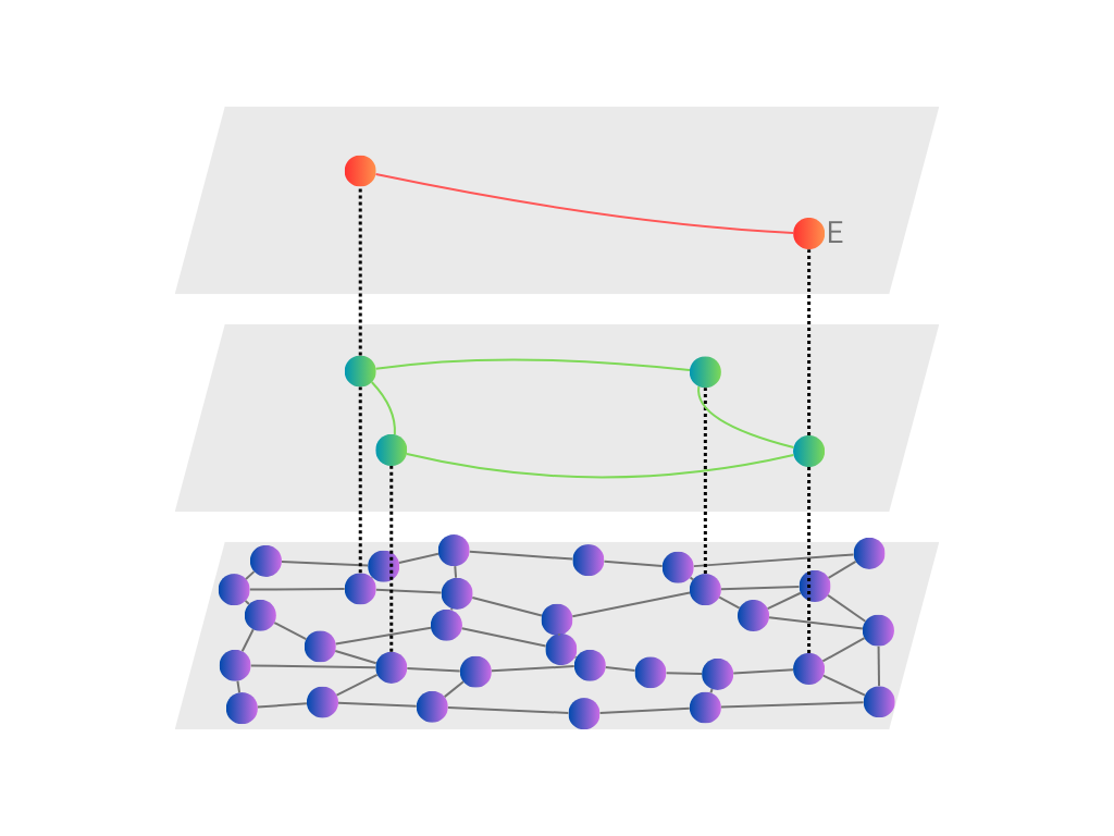
The idea of separate short and long connections can be generalised to include several intermediate levels of connection lengths. We can visualise this as a hierarchy of layers of connected vectors, with each layer only using a fraction of the vectors in the layer below.

The best number of layers (and other parameters like the maximum number of connections of each vector) can be found by experiment; there are also heuristics suggested in the HNSW paper.

Incidentally, HNSW also generalises another data structure called a skip list, which enables fast searching of sorted one-dimensional values (rather than multi-dimensional vectors).

Building an HNSW uses similar ideas to NSW. Vectors are inserted one at a time, and long-range connections are created through connecting random vectors — although in HNSW, these vectors are randomly chosen throughout the whole building process (while in NSW they were the first vectors in the random order of insertion).

To be precise, whenever a new vector is inserted, we first use a random function to choose the highest layer in which it will appear. All vectors appear in the bottom layer; a fraction of those also appear in the first layer up; a fraction of those also appear in the second layer up; and so on.

Similar to NSW, we then connect the inserted vector to its m nearest neighbours in each layer that it appears; we can search for these neighbours efficiently using the index built so far. As the vectors become more sparse in higher layers, the connections typically become longer.

Summary

This completes the discussion of the main ideas leading to HNSW. To summarise:

A small world is a graph that connects local points but also has short paths between distant points. This can be achieved through hubs with long-range connections.

Building these long-range connections in the right way results in a small world that is navigable, meaning a greedy algorithm can quickly find the short paths. This enables fast nearest neighbour search.

One such method for building the connections is to insert vectors in a random order and connect them to their nearest neighbours. However, this leads to long-range hubs with many connections, and a slower search time.

To avoid this, a better method is to separately build connections of different lengths by choosing random vectors to use as hubs. This gives us the HNSW index, which significantly increases the speed of nearest neighbour search.

Appendix

The post above provides an overview of the HNSW index and the ideas behind it. This appendix discusses additional interesting details of the HNSW algorithms for readers seeking a complete understanding. See the references for further details and pseudocode.

Improved search

Navigable small world methods only give approximate results for nearest neighbour search. Sometimes, the greedy search algorithm stops before finding the nearest vector to the target. This happens when the search path encounters a “false local optimum”, meaning the vector’s immediate connections are all further from the target, although there is a closer vector somewhere else in the graph.

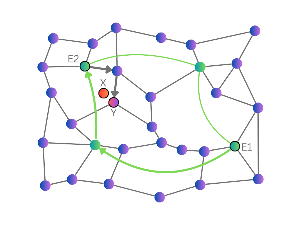
Things can be improved by performing several independent searches from different entry points, the results of which can give us several good candidates for the nearest neighbour. We then calculate the distance of all of the candidates to the target, and return the closest one.

If we want to find more than one (say k) nearest neighbours, we can first expand the set of candidates by adding all of their immediate connections, before calculating the distances to the target and returning the closest k.

This simple method for finding candidates has some shortcomings. Each greedy search path is still at risk of ending at a false local optimum; this could be improved by exploring beyond the immediate connections of each vector. Also, a search path may encounter several vectors towards the end which are close to the target, but aren’t chosen as candidates (because they aren’t the final vector in the path or one of its immediate connections).

Rather than following several greedy paths independently, a more effective approach is to follow a set of vectors, updating the whole set in a greedy fashion.

To be precise, we will maintain a set containing the closest vectors to the target encountered so far, along with their distances to the target. This set holds a maximum of ef vectors, where ef is the desired number of candidates. Initially, the set contains the entry points. We then proceed by a greedy process, evaluating each vector in the set by checking its connections.

All vectors in the set are initially marked as “unevaluated”. At each step, we evaluate the closest unevaluated vector to the target (and mark it as “evaluated”). Evaluating the vector means checking each of its connected vectors by calculating that vector’s distance to the target, and inserting it into the set (marked as “unevaluated”) if it’s closer than some of the vectors there (pushing the furthest vector out of the set if it’s at maximum capacity). (We also keep track of the vectors for which we’ve already calculated the distance, to avoid repeating work.)

The process ends when all of the vectors in the set have been evaluated and no new vectors have been inserted. The final set is returned as the candidates, from which we can take the closest vector or k closest vectors to the target.

(Note that for ef = 1, this algorithm is simply the basic greedy search algorithm.)

HNSW search & insertion

The above describes a search algorithm for an NSW, or a single layer of an HNSW.

To search the whole HNSW structure, the suggested approach is to use basic greedy search for the nearest neighbour in each layer from the top until we reach the layer of interest, at which point we use the layer search algorithm with several candidates.

For performing a k-nearest neighbours search (including k = 1) on the completed index, this means using basic greedy search until we reach the bottom layer, at which point we use the layer search algorithm with ef = efSearch candidates. efSearch is a parameter to be tuned; higher efSearch is slower but more accurate.

For inserting a vector into HNSW, we use basic greedy search until the first layer in which the new vector appears. Here, we search for the m nearest neighbours using layer search with ef = efConstruction candidates. We also use the candidates as the entry points for continuing the process in the next layer down.

Improved insertion

NSW introduced a simple method of building the graph in which each inserted vector is connected to its m nearest neighbours. While this method for choosing connections also works for HNSW, a modified approach was introduced which significantly improves the performance of the resulting index.

As usual, we start by finding efConstruction candidate vectors. We then go through these candidates in order of increasing distance from the inserted vector and connect them. However, if a candidate is closer to one of the newly connected candidates than it is to the inserted vector, we skip over it without connecting. We stop when m candidates have been connected.

The idea is that we can already reach the candidate from the inserted vector through a newly connected candidate, so it’s a waste to also add a direct connection; it’s better to connect a more distant point. This increases the diversity of connections in the graph, and helps connect nearby clusters of vectors.

References

[1] J. Travers and S. Milgram, An Experimental Study of the Small World Problem (1969), Sociometry

[2] J. Kleinberg, The Small-World Phenomenon: An Algorithmic Perspective (2000), Proceedings of the thirty-second annual ACM symposium on Theory of Computing

[3] Y. Malkov, A. Ponomarenko, A. Logvinov and V. Krylov, Approximate nearest neighbor algorithm based on navigable small world graphs (2014), Information Systems, vol. 45
(There are several similar papers; this one is the most recent and complete, and includes the more advanced k-nearest neighbours search algorithm.)

[4] Y. Malkov and D. Yashunin, Efficient and robust approximate nearest neighbor search using Hierarchical Navigable Small World graphs (2016), IEEE Transactions on Pattern Analysis and Machine Intelligence

All images are created by the author and free to use with a citation.

What’s The Story With HNSW? was originally published in Towards Data Science on Medium, where people are continuing the conversation by highlighting and responding to this story.

Exploring the path to fast nearest neighbour search with Hierarchical Navigable Small Worlds

Hierarchical Navigable Small World (HNSW) has become popular as one of the best performing approaches for approximate nearest neighbour search. HNSW is a little complex though, and descriptions often lack a complete and intuitive explanation. This post takes a journey through the history of the HNSW idea to help explain what “hierarchical navigable small world” actually means and why it’s effective.

Contents

• Approximate Nearest Neighbour Search
• Small Worlds
• Navigable Small Worlds
• Hierarchical Navigable Small Worlds
• Summary
• Appendix
  – Improved search
  – HNSW search & insertion
  – Improved insertion
• References

Approximate Nearest Neighbour Search

A common application of machine learning is nearest neighbour search, which means finding the most similar items* to a target — for example, to recommend items that are similar to a user’s preferences, or to search for items that are similar to a user’s search query.

The simple method is to calculate the similarity of every item to the target and return the closest ones. However, if there are a large number of items (maybe millions), this will be slow.

Instead, we can use a structure called an index to make things much faster.

There is a trade-off, however. Unlike the simple method, indexes only give approximate results: we may not retrieve all of the nearest neighbours (i.e. recall may be less than 100%).

There are several different types of index (e.g. locality sensitive hashing; inverted file index), but HNSW has proven particularly effective on various datasets, achieving high speeds while keeping high recall.

*Typically, items are represented as embeddings, which are vectors produced by a machine learning model; the similarity between items corresponds to the distance between the embeddings. This post will usually talk of vectors and distances, though in general HNSW can handle any kind of items with some measure of similarity.

Small Worlds

Small worlds were famously studied in Stanley Milgram’s small-world experiment [1].

Participants were given a letter containing the address and other basic details of a randomly chosen target individual, along with the experiment’s instructions. In the unlikely event that they personally knew the target, they were instructed to send them the letter; otherwise, they were told to think of someone they knew who was more likely to know the target, and send the letter on to them.

The surprising conclusion was that the letters were typically only sent around six times before reaching the target, demonstrating the famous idea of “six degrees of separation” — any two people can usually be connected by a small chain of friends.

In the mathematical field of graph theory, a graph is a set of points, some of which are connected. We can think of a social network as a graph, with people as points and friendships as connections. The small-world experiment found that most pairs of points in this graph are connected by short paths that have a small number of steps. (This is described technically as the graph having a low diameter.)

Having short paths is not that surprising in itself: most graphs have this property, including graphs created by just connecting random pairs of points. But social networks are not connected randomly, they are highly local: friends tend to live close to each other, and if you know two people, it’s quite likely they know each other too. (This is described technically as the graph having a high clustering coefficient.) The surprising thing about the small-world experiment is that two distant points are only separated by a short path despite connections typically being short-range.

In cases like these when a graph has lots of local connections, but also has short paths, we say the graph is a small world.

Another good example of a small world is the global airport network. Airports in the same region are highly connected to one another, but it’s possible to make a long journey in only a few stops by making use of major hub airports. For example, a journey from Manchester, UK to Osaka, Japan typically starts with a local flight from Manchester to London, then a long distance flight from London to Tokyo, and finally another local flight from Tokyo to Osaka. Long-range hubs are a common way of achieving the small world property.

A final interesting example of graphs with the small world property is biological neural networks such as the human brain.

Navigable Small Worlds

In small world graphs, we can quickly reach a target in a few steps. This suggests a promising idea for nearest neighbour search: perhaps if we create connections between our vectors in such a way that it forms a small world graph, we can quickly find the vectors near a target by starting from an arbitrary “entry point” vector and then navigating through the graph towards the target.

This possibility was explored by Kleinberg [2]. He noted that the existence of short paths wasn’t the only interesting thing about Miller’s experiment: it was also surprising that people were able to find these short paths, without using any global knowledge about the graph. Rather, the people were following a simple greedy algorithm. At each step, they examined each of their immediate connections, and sent it to the one they thought was closest to the target. We can use a similar algorithm to search a graph that connects vectors.

Kleinberg wanted to know whether this greedy algorithm would always find a short path. He ran simple simulations of small worlds in which all of the points were connected to their immediate neighbours, with additional longer connections created between random points. He discovered that the greedy algorithm would only find a short path in specific conditions, depending on the lengths of the long-range connections.

If the long-range connections were too long (as was the case when they connected pairs of points in completely random locations), the greedy algorithm could follow a long-range connection to quickly reach the rough area of the target, but after that the long-range connections were of no use, and the path had to step through the local connections to get closer. On the other hand, if the long-range connections were too short, it would simply take too many steps to reach the area of the target.

If, however, the lengths of the long-range connections were just right (to be precise, if they were uniformly distributed, so that all lengths were equally likely), the greedy algorithm would typically reach the neighbourhood of the target in an especially small number of steps (to be more specific, a number proportional to log(n), where n is the number of points in the graph).

In cases like this where the greedy algorithm can find the target in a small number of steps, we say the small world is a navigable small world (NSW).

An NSW sounds like an ideal index for our vectors, but for vectors in a complex, high-dimensional space, it’s not clear how to actually build one. Fortunately, Malkov et al. [3] discovered a method: we insert one randomly chosen vector at a time to the graph, and connect it to a small number m of nearest neighbours that were already inserted.

This method is remarkably simple and requires no global understanding of how the vectors are distributed in space. It’s also very efficient, as we can use the graph built so far to perform the nearest neighbour search for inserting each vector.

Experiments confirmed that this method produces an NSW. Because the vectors inserted early on are randomly chosen, they tend to be quite far apart. They therefore form the long-range connections needed for a small world. It’s not so obvious why the small world is navigable, but as we insert more vectors, the connections will get gradually shorter, so it’s plausible that the distribution of connection lengths will be fairly even, as required.

Hierarchical Navigable Small Worlds

Navigable small worlds can work well for approximate nearest neighbours search, but further analysis revealed areas for improvement, leading Markov et al. [4] to propose HNSW.

A typical path through an NSW from the entry point towards the target went through two phases: a “zoom-out” phase, in which connection lengths increase from short to long, and a “zoom-in” phase, in which the reverse happens.

The first simple improvement is to use a long-range hub (such as the first inserted vector) as the entry point. This way, we can skip the zoom-out phase and go straight to the zoom-in phase.

Secondly, although the search paths were short (with a number of steps proportional to log(n)), the whole search procedure wasn’t so fast. At each vector along the path, the greedy algorithm must examine each of the connected vectors, calculating their distance to the target in order to choose the closest one. While most of the locally connected vectors had only a few connections, most long-range hubs had many connections (again, a number proportional to log(n)); this makes sense as these vectors were usually inserted early on in the building process and had many opportunities to connect to other vectors. As a result, the total number of calculations during a search was quite large (proportional to log(n)²).

To improve this, we need to limit the number of connections checked at each hub. This leads to the main idea of HNSW: explicitly distinguishing between short-range and long-range connections. In the initial stage of a search, we will only consider the long-range connections between hubs. Once the greedy search has found a hub near the target, we then switch to using the short-range connections.

As the number of hubs is relatively small, they should have few connections to check. We can also explicitly impose a maximum number of long-range and short-range connections of each vector when we build the index. This results in a fast search time (proportional to log(n)).

The idea of separate short and long connections can be generalised to include several intermediate levels of connection lengths. We can visualise this as a hierarchy of layers of connected vectors, with each layer only using a fraction of the vectors in the layer below.

The best number of layers (and other parameters like the maximum number of connections of each vector) can be found by experiment; there are also heuristics suggested in the HNSW paper.

Incidentally, HNSW also generalises another data structure called a skip list, which enables fast searching of sorted one-dimensional values (rather than multi-dimensional vectors).

Building an HNSW uses similar ideas to NSW. Vectors are inserted one at a time, and long-range connections are created through connecting random vectors — although in HNSW, these vectors are randomly chosen throughout the whole building process (while in NSW they were the first vectors in the random order of insertion).

To be precise, whenever a new vector is inserted, we first use a random function to choose the highest layer in which it will appear. All vectors appear in the bottom layer; a fraction of those also appear in the first layer up; a fraction of those also appear in the second layer up; and so on.

Similar to NSW, we then connect the inserted vector to its m nearest neighbours in each layer that it appears; we can search for these neighbours efficiently using the index built so far. As the vectors become more sparse in higher layers, the connections typically become longer.

Summary

This completes the discussion of the main ideas leading to HNSW. To summarise:

A small world is a graph that connects local points but also has short paths between distant points. This can be achieved through hubs with long-range connections.

Building these long-range connections in the right way results in a small world that is navigable, meaning a greedy algorithm can quickly find the short paths. This enables fast nearest neighbour search.

One such method for building the connections is to insert vectors in a random order and connect them to their nearest neighbours. However, this leads to long-range hubs with many connections, and a slower search time.

To avoid this, a better method is to separately build connections of different lengths by choosing random vectors to use as hubs. This gives us the HNSW index, which significantly increases the speed of nearest neighbour search.

Appendix

The post above provides an overview of the HNSW index and the ideas behind it. This appendix discusses additional interesting details of the HNSW algorithms for readers seeking a complete understanding. See the references for further details and pseudocode.

Improved search

Navigable small world methods only give approximate results for nearest neighbour search. Sometimes, the greedy search algorithm stops before finding the nearest vector to the target. This happens when the search path encounters a “false local optimum”, meaning the vector’s immediate connections are all further from the target, although there is a closer vector somewhere else in the graph.

Things can be improved by performing several independent searches from different entry points, the results of which can give us several good candidates for the nearest neighbour. We then calculate the distance of all of the candidates to the target, and return the closest one.

If we want to find more than one (say k) nearest neighbours, we can first expand the set of candidates by adding all of their immediate connections, before calculating the distances to the target and returning the closest k.

This simple method for finding candidates has some shortcomings. Each greedy search path is still at risk of ending at a false local optimum; this could be improved by exploring beyond the immediate connections of each vector. Also, a search path may encounter several vectors towards the end which are close to the target, but aren’t chosen as candidates (because they aren’t the final vector in the path or one of its immediate connections).

Rather than following several greedy paths independently, a more effective approach is to follow a set of vectors, updating the whole set in a greedy fashion.

To be precise, we will maintain a set containing the closest vectors to the target encountered so far, along with their distances to the target. This set holds a maximum of ef vectors, where ef is the desired number of candidates. Initially, the set contains the entry points. We then proceed by a greedy process, evaluating each vector in the set by checking its connections.

All vectors in the set are initially marked as “unevaluated”. At each step, we evaluate the closest unevaluated vector to the target (and mark it as “evaluated”). Evaluating the vector means checking each of its connected vectors by calculating that vector’s distance to the target, and inserting it into the set (marked as “unevaluated”) if it’s closer than some of the vectors there (pushing the furthest vector out of the set if it’s at maximum capacity). (We also keep track of the vectors for which we’ve already calculated the distance, to avoid repeating work.)

The process ends when all of the vectors in the set have been evaluated and no new vectors have been inserted. The final set is returned as the candidates, from which we can take the closest vector or k closest vectors to the target.

(Note that for ef = 1, this algorithm is simply the basic greedy search algorithm.)

HNSW search & insertion

The above describes a search algorithm for an NSW, or a single layer of an HNSW.

To search the whole HNSW structure, the suggested approach is to use basic greedy search for the nearest neighbour in each layer from the top until we reach the layer of interest, at which point we use the layer search algorithm with several candidates.

For performing a k-nearest neighbours search (including k = 1) on the completed index, this means using basic greedy search until we reach the bottom layer, at which point we use the layer search algorithm with ef = efSearch candidates. efSearch is a parameter to be tuned; higher efSearch is slower but more accurate.

For inserting a vector into HNSW, we use basic greedy search until the first layer in which the new vector appears. Here, we search for the m nearest neighbours using layer search with ef = efConstruction candidates. We also use the candidates as the entry points for continuing the process in the next layer down.

Improved insertion

NSW introduced a simple method of building the graph in which each inserted vector is connected to its m nearest neighbours. While this method for choosing connections also works for HNSW, a modified approach was introduced which significantly improves the performance of the resulting index.

As usual, we start by finding efConstruction candidate vectors. We then go through these candidates in order of increasing distance from the inserted vector and connect them. However, if a candidate is closer to one of the newly connected candidates than it is to the inserted vector, we skip over it without connecting. We stop when m candidates have been connected.

The idea is that we can already reach the candidate from the inserted vector through a newly connected candidate, so it’s a waste to also add a direct connection; it’s better to connect a more distant point. This increases the diversity of connections in the graph, and helps connect nearby clusters of vectors.

References

[1] J. Travers and S. Milgram, An Experimental Study of the Small World Problem (1969), Sociometry

[2] J. Kleinberg, The Small-World Phenomenon: An Algorithmic Perspective (2000), Proceedings of the thirty-second annual ACM symposium on Theory of Computing

[3] Y. Malkov, A. Ponomarenko, A. Logvinov and V. Krylov, Approximate nearest neighbor algorithm based on navigable small world graphs (2014), Information Systems, vol. 45
(There are several similar papers; this one is the most recent and complete, and includes the more advanced k-nearest neighbours search algorithm.)

[4] Y. Malkov and D. Yashunin, Efficient and robust approximate nearest neighbor search using Hierarchical Navigable Small World graphs (2016), IEEE Transactions on Pattern Analysis and Machine Intelligence

All images are created by the author and free to use with a citation.

What’s The Story With HNSW? was originally published in Towards Data Science on Medium, where people are continuing the conversation by highlighting and responding to this story.

FOLLOW US ON GOOGLE NEWS

Read original article here