
When R Meets SQL to Query Dataframes | by Zoumana Keita | Jun, 2022
A comprehensive overview of running SQL commands on R Dataframes
As a Data Scientist, you might already hear of SQL and R. SQL is great for interacting with relational databases. R on the other hand is a great tool for performing advanced statistical analysis. However, some tasks are simpler in SQL than in R, and vice-versa. What if we could have a tool that can combine the beauty of each tool? That is where sqldfcomes in handy. This article aims to highlight some features of sqldf , similar to those in SQL.
sqldf is an open-source library used to run SQL Statements on R data frames. It works with multiple databases such as SQLite, H2, PostgreSQL, and MySQL databases.
Install the packages
Time to get started with the hands-on! But, we first need to install the sqldf library using the install.packages function.
# Install the library
install.packages("sqldf") # Load the library
library("sqldf")
Data & Preprocessing
In this article, we will use one of the standard machine learning datasets known as the “Adult Income” freely available under the UCI Machine Learning license. Start by getting the dataset either by reading straight from my Github or downloading and save in your current working directory using the read.csv() function.
data_url = "https://raw.githubusercontent.com/keitazoumana/Medium-Articles-Notebooks/main/data/adult-all.csv"# Read the data
income_data <- read.csv(data_url)# Check the first 5 rows of the data
head(income_data, 5)
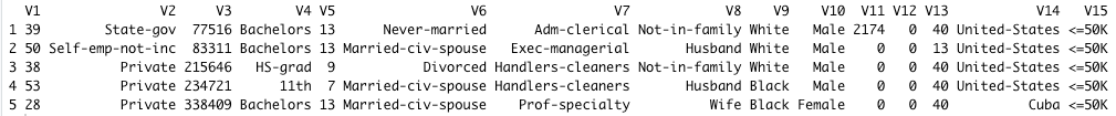
The columns (V1, V1, …, V15) of the data are not understandable, we can rename them with the following syntax. These names come from the UCI Machine Learning website, so nothing is invented.
new_columns = c("Age", "Workclass", "fnlwgt", "Education", "EducationNum", "MartialStatus", "Occupation",
"Relationship", "Race", "Sex", "CapitalGain",
"CapitalLoss", "HoursPerWeek", "Country", "Income")# Change column names
colnames(income_data) <- new_columns# Check the first 5 rows of the data again
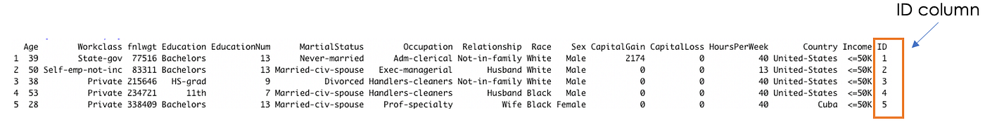
head(income_data, 5)

The changes have been successfully performed, as you can see in the previous screenshot.
To finish, let’s add an ID column to the data set using the tidy, which will be the identifier of each person. You will find the benefit of this column later in the article.
# Add the ID column to the dataset
income_data$ID <- 1:nrow(income_data)# Show the first 5 rows
To be able to perform any SQL query, you need to use the sqldf function, which takes as a parameter your query in string format, as shown below.
sqldf("YOUR_SQL_QUERY")
In this section, we will cover different queries from simple to more advanced ones, starting with columns selection.
Columns selection
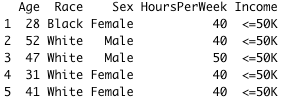
We can retrieve data columns satisfying one or multiple conditions. For instance, we can extract the Age, Race, Sex, HoursPerWeek, and Income of adults from Cuba.
Note: In the syntax, make sure to not forget the ‘ ‘ sign around Cuba to make it work.
cuba_query = "SELECT Age, Race, Sex, HoursPerWeek, Income \
FROM income_data \
WHERE Country = 'Cuba'"
cuba_data = sqldf(cuba_query)
head(cuba_data, 5)
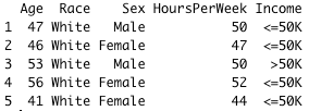
We might want to add an additional constraint in order to get only Cuban adults who work more than 40 hours a week and who are less than 40 years old.
cuba_query_2 = "SELECT Age, Race, Sex, HoursPerWeek, Income \
FROM income_data \
WHERE Country = 'Cuba'\
AND HoursPerWeek > 40 \
AND Age > 40"cuba_data_2 = sqldf(cuba_query_2)
head(cuba_data_2, 5)
GROUP BY Statement
In addition to selecting columns, we might also want to partition our data into different groups in order to get a more general overview with the help of functions such as AVG(), COUNT(), MAX(), MIN(), and SUM(). Using GROUP BY, a particular column with the same values in different rows will be grouped together.
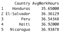
For instance, let’s consider taking the average number of weekly working hours per country and then sort in increasing order of average working hours.
# Prepare the query
wwh_per_country_query = "SELECT Country, AVG(HoursPerWeek)
AS AvgWorkHours \
FROM income_data
GROUP BY Country
ORDER BY AvgWorkHours ASC"# Run the query
wwh_per_country_data = sqldf(wwh_per_country_query) # Get the first 5 observations
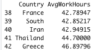
head(wwh_per_country_data, 5)# Get the last 5 observations
tail(wwh_per_country_data, 5)
Let’s break down the query for better clarification.
SELECT Country, AVG(HoursPerWeek) AS AvgWorkHours: we select all the countries and their respective weekly hours. Then the result of the average hours is computed with theAVGfunction, and stored in a new column called AvgWorkHours.GROUP BY Country: at the end of the previous statement, all the countries with the same name will have the same result of AvgWorkHours. GROUP BY is then used to create a unique instance of each country with their corresponding AvgWorkHours.ORDER BY AvgWorkHours ASC: this final statement is used to sort the AvgWorkHours in increasing order using theASC(ascending) function.
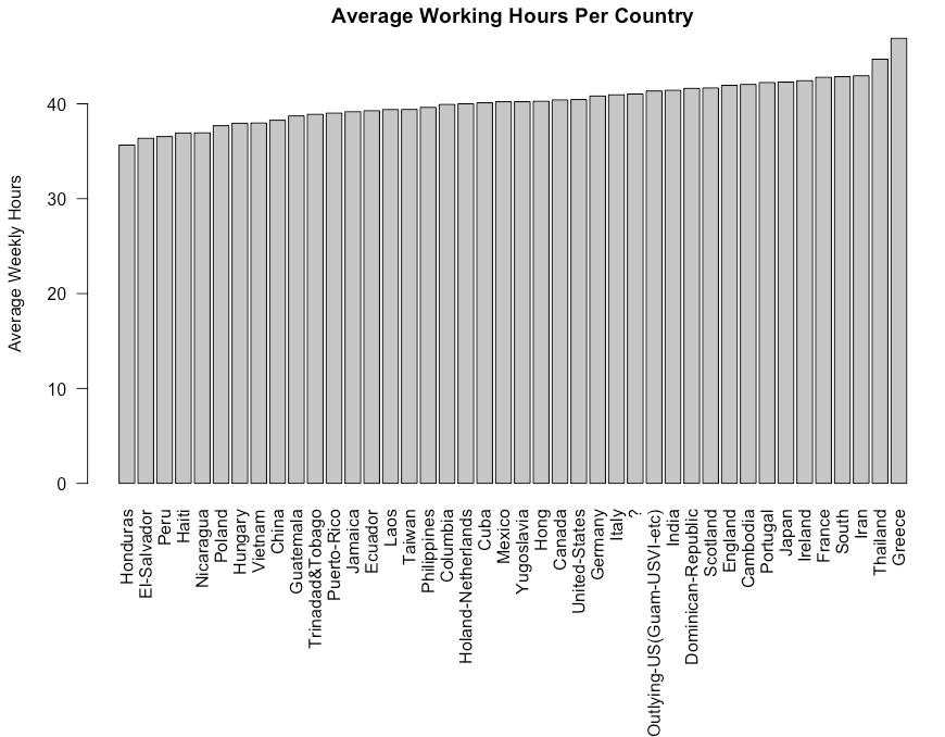
If you are a more graphical person, you can show the previous result using pure R scripts. Switching from R to SQL! Isn’t that amazing 🙂
# Create a plot# Create room for the plot
graphics.off()# Sets or adjusts plotting parameters
par("mar")
par(mar = c(12, 4, 2, 2) + 0.2)# Show the final plot
barplot(height = wwh_per_country_data$AvgWorkHours,
names.arg = wwh_per_country_data$Country,
main ="Average Working Hours Per Country",
ylab = "Average Weekly Hours",
las = 2)
par()function is used to adjust the plotting parameters, andmaris a vector of length 4, and sets the margin sizes respectively for the bottom, left, top, and right.las=2is used to show Country names in a vertical way for better visualization. A value of 1 would show them horizontally.
It is only what sqldf is capable of? Just column selection and Group by?
Of course not! There are much more SQL queries that can be performed. Let’s finish this article with the use of JOINS.
JOINS Statement
Those are used to combine rows from at least two data sets (i.e. tables), based on column(s) that link those tables. To successfully demonstrate this scenario, we need to create an additional data set.
Data sets creation
Let’s start by creating two different data sets.
- The first one is called
personal_info_datawhich will contain all the personal information about a person. - The second one is named
backg_info_datawhich will contain all the academic, salary information, etc.
# Prepare the query
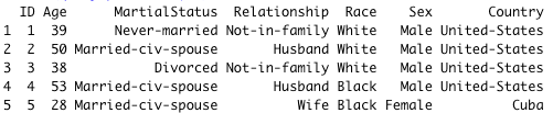
query_pers_info = "SELECT ID, Age, MartialStatus, Relationship, Race, Sex, Country FROM income_data"# Store the result in the personal_info_data variable
personal_info_data = sqldf(query_pers_info)# Show the first 5 rows of the result
head(personal_info_data, 5)
Creating the second one uses a similar approach to the previous one.
# Prepare the query
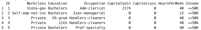
query_backg_info = "SELECT ID,Workclass, Education, Occupation, CapitalGain, CapitalLoss, HoursPerWeek, Income FROM income_data"# Store the result in the backg_info_data variable
backg_info_data = sqldf(query_backg_info)# Show the first 5 rows of the result
head(backg_info_data, 5)
Notice that the ID in the personal_info_data refers to the ID in backg_info_data . Thus, the relationship between our two data sets is the ID column. sqldf can execute all different types of joins, but our focus will be on the INNER JOIN, which returns all the records that have matching values in both tables.
The following statement extracts adults’ age, marital status, country, education, and income.
# Prepare the query
join_query = "SELECT p_info.ID, \
p_info.Age, \
p_info.MartialStatus, \
p_info.Country, \
bg_info.Education,\
bg_info.Income \
FROM personal_info_data p_info \
INNER JOIN backg_info_data bg_info \
ON p_info.ID = bg_info.ID"# Run the qery
join_data = sqldf(join_query)# Show the first 5 observations
head(join_data, 5)
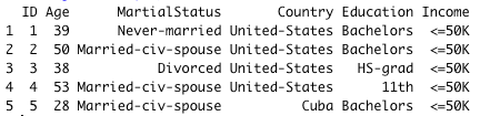
The query has been broken down with the creation of additional variables for clarification and readability sake.
sp_info: it would be too long to write personal_info_data.Education, personal_info_data.MaritalStatus, etc. We create an alias/instance that can be used instead of the original name. The alias most of the time is shorter than the original one.bg_info:similarly to the previous one is an alias of backg_info_data.
No R users are left behind! 🎉 🍾 You have just learned how to use sqldf to interact with your R data frames. If you are still performing complicated tasks that might be easier with SQL, now is the time to give sqldf a try, it might help you and your colleagues save time and be more productive!
Also, If you like reading my stories and wish to support my writing, consider becoming a Medium member to unlock unlimited access to stories on Medium. By doing so, I’ll receive a small commission.
Feel free to follow me on Medium, Twitter, or say Hi on LinkedIn. It is always a pleasure to discuss AI, ML, Data Science, NLP, and MLOps stuff!
A comprehensive overview of running SQL commands on R Dataframes

As a Data Scientist, you might already hear of SQL and R. SQL is great for interacting with relational databases. R on the other hand is a great tool for performing advanced statistical analysis. However, some tasks are simpler in SQL than in R, and vice-versa. What if we could have a tool that can combine the beauty of each tool? That is where sqldfcomes in handy. This article aims to highlight some features of sqldf , similar to those in SQL.
sqldf is an open-source library used to run SQL Statements on R data frames. It works with multiple databases such as SQLite, H2, PostgreSQL, and MySQL databases.
Install the packages
Time to get started with the hands-on! But, we first need to install the sqldf library using the install.packages function.
# Install the library
install.packages("sqldf") # Load the library
library("sqldf")
Data & Preprocessing
In this article, we will use one of the standard machine learning datasets known as the “Adult Income” freely available under the UCI Machine Learning license. Start by getting the dataset either by reading straight from my Github or downloading and save in your current working directory using the read.csv() function.
data_url = "https://raw.githubusercontent.com/keitazoumana/Medium-Articles-Notebooks/main/data/adult-all.csv"# Read the data
income_data <- read.csv(data_url)# Check the first 5 rows of the data
head(income_data, 5)
The columns (V1, V1, …, V15) of the data are not understandable, we can rename them with the following syntax. These names come from the UCI Machine Learning website, so nothing is invented.
new_columns = c("Age", "Workclass", "fnlwgt", "Education", "EducationNum", "MartialStatus", "Occupation",
"Relationship", "Race", "Sex", "CapitalGain",
"CapitalLoss", "HoursPerWeek", "Country", "Income")# Change column names
colnames(income_data) <- new_columns# Check the first 5 rows of the data again
head(income_data, 5)
The changes have been successfully performed, as you can see in the previous screenshot.
To finish, let’s add an ID column to the data set using the tidy, which will be the identifier of each person. You will find the benefit of this column later in the article.
# Add the ID column to the dataset
income_data$ID <- 1:nrow(income_data)# Show the first 5 rows
To be able to perform any SQL query, you need to use the sqldf function, which takes as a parameter your query in string format, as shown below.
sqldf("YOUR_SQL_QUERY")
In this section, we will cover different queries from simple to more advanced ones, starting with columns selection.
Columns selection
We can retrieve data columns satisfying one or multiple conditions. For instance, we can extract the Age, Race, Sex, HoursPerWeek, and Income of adults from Cuba.
Note: In the syntax, make sure to not forget the ‘ ‘ sign around Cuba to make it work.
cuba_query = "SELECT Age, Race, Sex, HoursPerWeek, Income \
FROM income_data \
WHERE Country = 'Cuba'"
cuba_data = sqldf(cuba_query)
head(cuba_data, 5)
We might want to add an additional constraint in order to get only Cuban adults who work more than 40 hours a week and who are less than 40 years old.
cuba_query_2 = "SELECT Age, Race, Sex, HoursPerWeek, Income \
FROM income_data \
WHERE Country = 'Cuba'\
AND HoursPerWeek > 40 \
AND Age > 40"cuba_data_2 = sqldf(cuba_query_2)
head(cuba_data_2, 5)
GROUP BY Statement
In addition to selecting columns, we might also want to partition our data into different groups in order to get a more general overview with the help of functions such as AVG(), COUNT(), MAX(), MIN(), and SUM(). Using GROUP BY, a particular column with the same values in different rows will be grouped together.
For instance, let’s consider taking the average number of weekly working hours per country and then sort in increasing order of average working hours.
# Prepare the query
wwh_per_country_query = "SELECT Country, AVG(HoursPerWeek)
AS AvgWorkHours \
FROM income_data
GROUP BY Country
ORDER BY AvgWorkHours ASC"# Run the query
wwh_per_country_data = sqldf(wwh_per_country_query) # Get the first 5 observations
head(wwh_per_country_data, 5)# Get the last 5 observations
tail(wwh_per_country_data, 5)
Let’s break down the query for better clarification.
SELECT Country, AVG(HoursPerWeek) AS AvgWorkHours: we select all the countries and their respective weekly hours. Then the result of the average hours is computed with theAVGfunction, and stored in a new column called AvgWorkHours.GROUP BY Country: at the end of the previous statement, all the countries with the same name will have the same result of AvgWorkHours. GROUP BY is then used to create a unique instance of each country with their corresponding AvgWorkHours.ORDER BY AvgWorkHours ASC: this final statement is used to sort the AvgWorkHours in increasing order using theASC(ascending) function.
If you are a more graphical person, you can show the previous result using pure R scripts. Switching from R to SQL! Isn’t that amazing 🙂
# Create a plot# Create room for the plot
graphics.off()# Sets or adjusts plotting parameters
par("mar")
par(mar = c(12, 4, 2, 2) + 0.2)# Show the final plot
barplot(height = wwh_per_country_data$AvgWorkHours,
names.arg = wwh_per_country_data$Country,
main ="Average Working Hours Per Country",
ylab = "Average Weekly Hours",
las = 2)
par()function is used to adjust the plotting parameters, andmaris a vector of length 4, and sets the margin sizes respectively for the bottom, left, top, and right.las=2is used to show Country names in a vertical way for better visualization. A value of 1 would show them horizontally.
It is only what sqldf is capable of? Just column selection and Group by?
Of course not! There are much more SQL queries that can be performed. Let’s finish this article with the use of JOINS.
JOINS Statement
Those are used to combine rows from at least two data sets (i.e. tables), based on column(s) that link those tables. To successfully demonstrate this scenario, we need to create an additional data set.
Data sets creation
Let’s start by creating two different data sets.
- The first one is called
personal_info_datawhich will contain all the personal information about a person. - The second one is named
backg_info_datawhich will contain all the academic, salary information, etc.
# Prepare the query
query_pers_info = "SELECT ID, Age, MartialStatus, Relationship, Race, Sex, Country FROM income_data"# Store the result in the personal_info_data variable
personal_info_data = sqldf(query_pers_info)# Show the first 5 rows of the result
head(personal_info_data, 5)
Creating the second one uses a similar approach to the previous one.
# Prepare the query
query_backg_info = "SELECT ID,Workclass, Education, Occupation, CapitalGain, CapitalLoss, HoursPerWeek, Income FROM income_data"# Store the result in the backg_info_data variable
backg_info_data = sqldf(query_backg_info)# Show the first 5 rows of the result
head(backg_info_data, 5)
Notice that the ID in the personal_info_data refers to the ID in backg_info_data . Thus, the relationship between our two data sets is the ID column. sqldf can execute all different types of joins, but our focus will be on the INNER JOIN, which returns all the records that have matching values in both tables.
The following statement extracts adults’ age, marital status, country, education, and income.
# Prepare the query
join_query = "SELECT p_info.ID, \
p_info.Age, \
p_info.MartialStatus, \
p_info.Country, \
bg_info.Education,\
bg_info.Income \
FROM personal_info_data p_info \
INNER JOIN backg_info_data bg_info \
ON p_info.ID = bg_info.ID"# Run the qery
join_data = sqldf(join_query)# Show the first 5 observations
head(join_data, 5)
The query has been broken down with the creation of additional variables for clarification and readability sake.
sp_info: it would be too long to write personal_info_data.Education, personal_info_data.MaritalStatus, etc. We create an alias/instance that can be used instead of the original name. The alias most of the time is shorter than the original one.bg_info:similarly to the previous one is an alias of backg_info_data.
No R users are left behind! 🎉 🍾 You have just learned how to use sqldf to interact with your R data frames. If you are still performing complicated tasks that might be easier with SQL, now is the time to give sqldf a try, it might help you and your colleagues save time and be more productive!
Also, If you like reading my stories and wish to support my writing, consider becoming a Medium member to unlock unlimited access to stories on Medium. By doing so, I’ll receive a small commission.
Feel free to follow me on Medium, Twitter, or say Hi on LinkedIn. It is always a pleasure to discuss AI, ML, Data Science, NLP, and MLOps stuff!
Denial of responsibility! Techno Blender is an automatic aggregator of the all world’s media. In each content, the hyperlink to the primary source is specified. All trademarks belong to their rightful owners, all materials to their authors. If you are the owner of the content and do not want us to publish your materials, please contact us by email – [email protected]. The content will be deleted within 24 hours.