A Comprehensive Guide to Modeling Techniques in Mixed-Integer Linear Programming

Convert ideas into mathematical expressions to solve operations research problems

Numerical optimization is at the core of quantitative techniques in decision science. It encompasses a set of frameworks to optimize one or more objectives under some prescribed set of circumstances.

Two major categories of optimization problems are Linear and Nonlinear Programming. These categories are distinguished by how the mathematical relationships between the decision variables are established in the objective(s) and constraints. Management sciences and operations research make extensive use of linear models, whereas nonlinear programming problems tend to arise naturally in the physical sciences and engineering (Nocedal & Wright, 2006).

Mathematical models often require the incorporation of discrete decisions and integer values. These have been especially explored in the context of linear models as efficient algorithms were proposed throughout the years. When a Linear Program (LP) includes integrality constraints, it is classified as an Integer or a Mixed-Integer Linear Program (MILP). Fortunately, we have several solvers available to solve these problems, including open-source alternatives such as HiGHS and SCIP.

Although mathematical models are imperfect representations of reality, they can be useful in guiding decisions. Therefore, this article aims to address how to describe common formulations and expressions encountered in MILP in mathematical terms.

The following sections will cover:

• Logical statements
• Setup costs and batch sizes
• Conditional expressions
• Discrete planning horizons
• Linearization techniques
• Further reading
• Conclusions
• References

This article will be a more abstract text on mathematical models than a code-applied guide. However, you might find several practical examples of how to solve numerical optimization models in my GitHub repository.

Before you start, remember you might have a better understanding of this text if you are already familiar with Linear Programming. You can find an interesting overview of the subject in my previous article.

Linear programming: Theory and applications

Now let us dive in!

Logical statements

In integer programming (IP) models, logical statements can be translated into linear constraints to capture specific conditions or relationships among the decision variables. Let us consider at first logical statements involving binary decision variables.

Implications

Let us start with the statement “if x then y”. It must ensure that if x is True (value of 1), y must also be True. Otherwise, y can be either 0 or 1. It can be described by a simple inequality stating that y is greater than or equal to x.

Logical NOT

The expression for “not y” must return its opposite. So, in case y is 1, it must return 0. Otherwise, it should return 1.

The “not” statement can be combined with an implication constraint, for instance, “if x then not y”.

Logical AND

To compute the logical “and”, let us introduce a variable z, which is True if both x and y are True. These are the same rules to describe the product between two binary variables, as x times y only equals 1 if both are equal to 1. This occurs in the Facility Dispersion Problem when computing an active edge connecting two nodes.

Logical OR

Now, to compute the logical “or”, z must be True if either x or y is True. We must then ensure that it is greater than or equal to each of them and that it is smaller than their sum.

Setup costs and batch sizes

Next, let us introduce setup costs and batch sizes, which are similar to implication constraints but in a context with real-valued and integer/binary variables. Consider a nonnegative variable x and a condition where setup costs apply if x is greater than zero. To mathematically represent this, we state that y multiplied by a large value M should be greater than or equal to x.

If x is greater than zero, the inequality is only satisfied if y is 1. This occurs for instance in the Dynamic Lot-size Problem, in which we balance between setup and holding inventory costs.

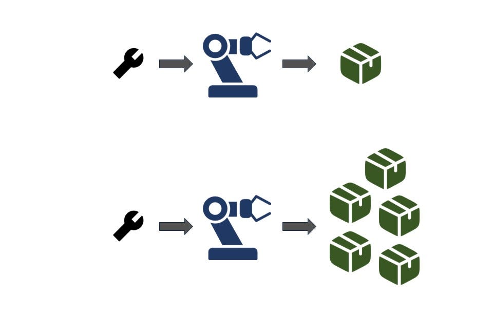
The M term — usually denoted the “big M” — should be a natural upper bound for x. It is important to define it using the smallest possible value such that the constraint is nonbinding if y equals 1. Avoiding too large values can improve linear relaxation, which has a positive effect on solver performance, besides avoiding numerical errors.

For scenarios involving multiple integer batches with limited capacity each (e.g., supply trips to a customer) we can use a similar expression. Now consider y is an integer variable denoting the number of batches performed and Q the capacity of each. The decision variable x still represents a nonnegative real value. We can write the same equation to capture our decision rules.

Conditional Expressions — “if-then” rules

Now imagine we want an inequality to be binding when a binary variable y is 1, else nonbinding. Once again, we can include a large value M to capture this condition.

In case y equals 1, the term multiplying M becomes zero and the original constraint is binding. Otherwise, M is multiplied by 1, therefore it assumes an arbitrarily large value such that the original constraint is nonbinding for any feasible value of x considering the context of the problem.

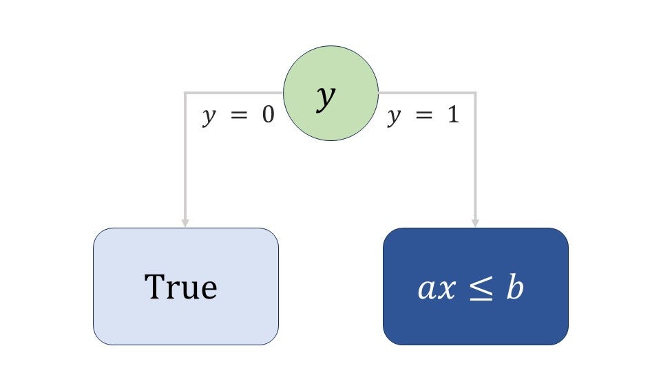
These expressions will arise quite often in mixed-integer programming models, and some of the most common applications are detailed here.

Disjunctive rules — “if-then-else”

Disjunctive constraints are a series of connected “if-then” constraints. Additional rules ensure that either one or the other is satisfied.

Precedence and sequences

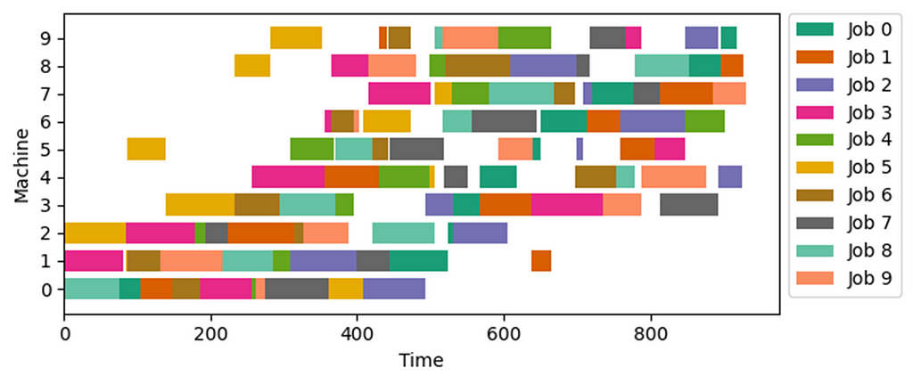
Consider now a decision as to which operation, i or j, happens first. In some sequencing models, we can include a real-valued decision variable for the start of each operation x, another variable or a fixed parameter for its duration d, and a binary decision variable (precedence) y which is 1 if i occurs before j.

These expressions will be useful in the Disjunctive Job-shop Scheduling Model and the Traveling Salesman Problem using the MTZ Formulation (Miller et al., 1960).

Min-max and Max-min objectives

These objectives involve the minimization of the maximum value of a set of expressions or the maximization of their minimum value. In simple terms, our goal is to keep the worst-case scenario as good as possible.

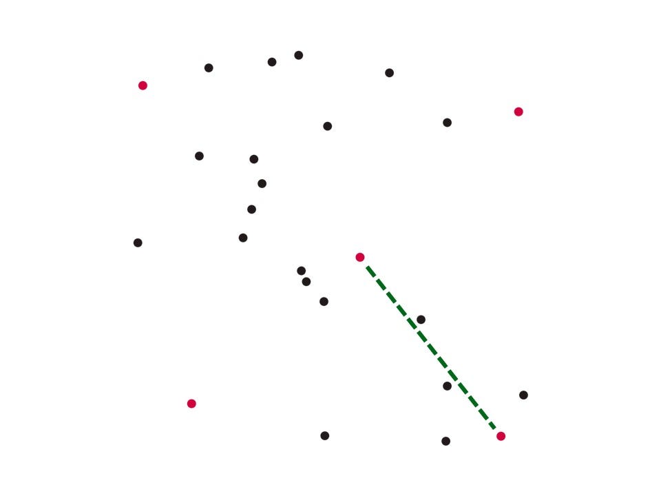
In the case of the Min-max expressions, we can create a scalar decision variable z and ensure that it is always greater than or equal to attributes d from a set of options I if the corresponding item i is selected.

When handling Max-min expressions, consider now z a scalar lesser than or equal to the attributes of all selected items. In both scenarios, we introduce the big M to ensure that, in case the item is not selected, the constraint becomes nonbinding. A good choice of M would be the difference between the maximum value of d (from the whole set of items) and the property of item i.

These expressions arise for instance in the Facility Dispersion Problem considering binary variables to indicate that a given arc or edge is active.

Discrete planning horizons

Several operations research problems include planning over a discrete horizon. In such situations, actions taken at a given moment from the timeline will affect how decisions should be performed in the future. For instance, production and inventory planning usually includes balancing between holding inventory costs, setup costs, stock coverage, and demand forecast, among other aspects. The amount produced of a given product at a given moment is usually a decision to be taken and it should affect the product availability not only when produced but also in the future when considering the possibility of stocking goods.

Inventory balance

To calculate inventory balance, let us define a discrete planning horizon T with instants t. The inventory at a given moment will be a decision variable I indexed by the elements of the set T. If we define inputs (for instance the number of items produced) and outputs (corresponding demand or items transported) of a given moment as x and d respectively, we can compute the final inventory at a given moment as the final inventory of the previous moment plus inputs minus outputs.

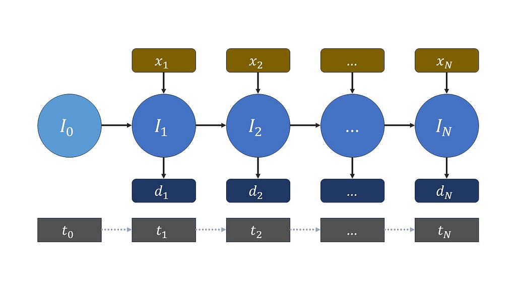
Remember the inputs and outputs might be fixed parameters of the problem or also decision variables.

We can put it in equation form as the following.

A great example to illustrate this is the Dynamic Lot-Size model. However, more complex decisions might be involved in the process and new elements should be included in the inventory balance equations then. One example will be presented right next.

Inventory with backlogs

Now suppose we have deterministic demands d for each moment t, but we might decide to postpone some of them to reduce our costs (for instance setup costs or fixed charges in transportation systems). These might become backlogs in an inventory balance equation, usually with some associated cost in the objective function(s). Once again consider our inputs are represented by x, but now we are also going to include a non-negative decision variable for backlogs b, also indexed by t. The new inventory balance equation becomes the following.

Then it is up to the optimization solver to define when a demand should be postponed to reduce overall costs.

Starts and Endings

Some planning processes include scheduling activities that start at a certain moment and might last for more than one instant in the discrete planning horizon. When inserting these decisions in an optimization model, usually it is up to the model to define when the activity starts, when it ends, and possibly its corresponding duration. Therefore, we must include some binary decision variables to represent these decisions.

To a better understanding of the modeling expressions, let us visually represent an activity that starts at a given moment, is active during some instants of the planning horizon, and then ends.

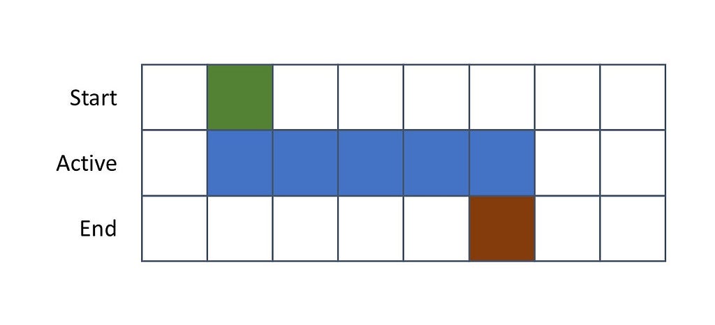
Notice that an activity starts in a moment in which it is active but it must be inactive in the previous instant. Conversely, at its ending, there’s no rule regarding the previous instant but it must be inactive in the following one.

To write that into mathematical expressions, let us use three groups of decision variables — all of them indexed by the elements of the planning horizon T. The variable x will be used to denote a moment in which the activity is active, y will denote its start, and z denote its ending.

To obtain a tight linear relaxation and help the solver during Branch & Bound, three groups of constraints will be created to establish the relationship between x and y, and the same between x and z.

To identify starts:

And to identify endings:

Additional implication constraints might be included in the first and last instants to ensure the desired relationships between x, y, and z in these moments.

Linearization techniques

Some problems include nonlinear expressions that cannot be incorporated directly into a MILP model. Fortunately, there are strategies involving the use of binary variables that allow us to linearize some nonlinear expressions. Two usual applications will be presented right next.

Product of real-valued and binary variables

Now, suppose we have a continuous decision variable x bounded between feasible limits L and U. Also suppose a binary decision variable y and a support decision variable z which should compute the product between x and y. When y is 1, z should assume the value of x, otherwise 0.

If y is 1, z must be greater than or equal to x (and its natural lower limit) and also lesser than or equal to x (and its natural upper limit). The only way to satisfy these inequalities is, therefore, if z is equal to x.

Now if y is 0, the last two inequalities ensure that z equals 0, while the first two inequalities ensure that any value of x between its natural bounds is feasible.

Therefore, using these inequalities, one can linearize the product between a binary and a real-valued decision variable.

Piecewise linear approximations

Now suppose we want to compute the value of a function defined in piecewise linear segments. It can be an approximation for a general nonlinear expression or simply a strategy to compute segmented linear expressions such as in contracts with distinct levels of unitary costs varying according to the volume of transactions. The idea is illustrated below by the approximation of the sigmoid function by 5 linear segments.

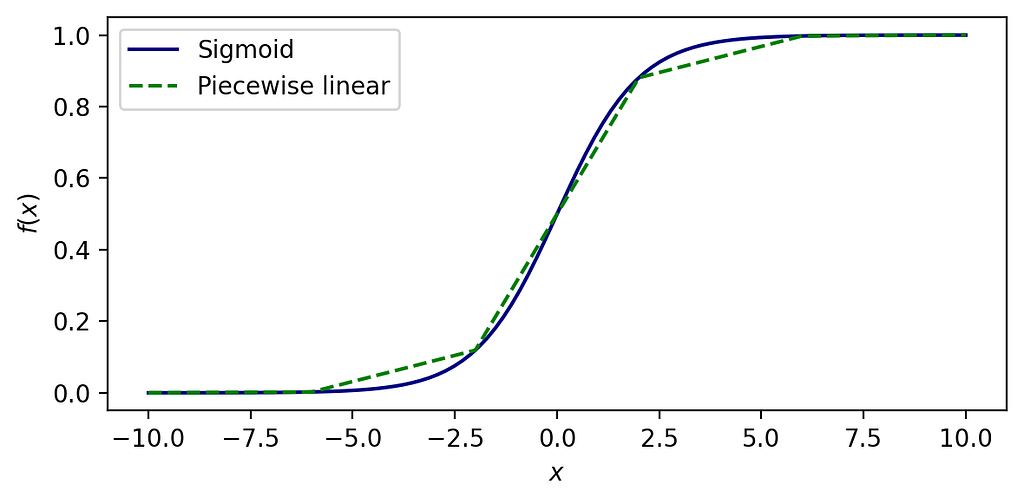
Consider a generic function f(x) defined in a given domain of a real-valued variable x between l and u. Now consider this function is discretized over N segments of arbitrary size. Each segment of index i lies between interpolation points x of indexes i and i+1, such that there are N+1 interpolation points. We now include parameters to define the linear equation of each segment:

• aᵢ: the slope of the ith linear segment
• bᵢ: the intercept of the ith linear segment

Our goal is that the decision variable y assumes the value of f(x). To do so, we also include auxiliary decision variables index by i within {1, 2, …, N}:

• zᵢ: a binary decision variable that is an indicator that x lies within the ith linear segment (closed interval).
• sᵢ: a real-valued decision variable that assumes the value of x in case it lies within the ith linear segment (closed interval).

The variable x should lie within one of the segments created, therefore a constraint must ensure that exactly one z variable is active.

Now we must ensure that sᵢ equals x when zᵢ equals 1, and also compute y based on the values of sᵢ and the corresponding parameters of each segment.

Thus, using these expressions one can compute the value of a generic piecewise linear function f(x) to a real-valued decision variable y in a way that a mixed-integer linear programming solver can interpret.

Further reading

The algorithm at the core of most MILP solvers is called Branch & Bound. It efficiently explores a rooted search tree of discrete decisions without enumerating all possibilities. You might find a comprehensive introduction to this topic in my previous article.

A Gentle Introduction to Branch & Bound

Some models might resort to other techniques, such as Delayed Column Generation, which aims to solve models with a number of decision variables too large to be explicitly enumerated from the start. An introduction on this topic with a coding example can be found in a previous article too.

Column Generation in Linear Programming and the Cutting Stock Problem

Now referring to traditional books on the subject, the interested reader might refer to Numerical Optimization (Nocedal & Wright, 2006) and Linear and Nonlinear Programming (Luenberger & Ye, 2008) for a deeper understanding of optimization algorithms over continuous domain — which are often components of submodels solved in integer programming. The book Integer Programming (Wolsey, 2020) is often referred to as “the bible” of its corresponding subject. It is a great reference to understand better how exact algorithms on discrete search spaces are designed going deeper into Branch & Bound, cutting planes, and much more. The book Operations research: applications and algorithms (Winston & Goldberg, 2004) is a great alternative for those eager to see more applied examples besides a great overview of theoretical aspects.

Conclusions

Mixed-Integer Linear Programming (MILP) is a relevant area in numerical optimization with relevant applications, especially in management sciences and operations research. This article covered key expressions of MILP including Logical statements, Setup costs, Conditional expressions, Discrete planning horizons, and Linearization techniques. By combining these elements, the reader should be able to formulate real-world problems as optimization models that can be tackled by MILP solvers.

References

Luenberger, D. G. & Ye, Y., 2008. Linear and Nonlinear Programming. 3rd ed. Stanford: Springer.

Nocedal, J. & Wright, S. J., 2006. Numerical Optimization. 2nd ed. New York: Springer New York.

Winston, W. L. & Goldberg, J. B., 2004. Operations research: applications and algorithms. 4th ed. Belmont, CA: Thomson Brooks/Cole Belmont.

Wolsey, L. A., 2020. Integer Programming. 2nd ed. John Wiley & Sons.

A Comprehensive Guide to Modeling Techniques in Mixed-Integer Linear Programming was originally published in Towards Data Science on Medium, where people are continuing the conversation by highlighting and responding to this story.

Convert ideas into mathematical expressions to solve operations research problems

Numerical optimization is at the core of quantitative techniques in decision science. It encompasses a set of frameworks to optimize one or more objectives under some prescribed set of circumstances.

Two major categories of optimization problems are Linear and Nonlinear Programming. These categories are distinguished by how the mathematical relationships between the decision variables are established in the objective(s) and constraints. Management sciences and operations research make extensive use of linear models, whereas nonlinear programming problems tend to arise naturally in the physical sciences and engineering (Nocedal & Wright, 2006).

Mathematical models often require the incorporation of discrete decisions and integer values. These have been especially explored in the context of linear models as efficient algorithms were proposed throughout the years. When a Linear Program (LP) includes integrality constraints, it is classified as an Integer or a Mixed-Integer Linear Program (MILP). Fortunately, we have several solvers available to solve these problems, including open-source alternatives such as HiGHS and SCIP.

Although mathematical models are imperfect representations of reality, they can be useful in guiding decisions. Therefore, this article aims to address how to describe common formulations and expressions encountered in MILP in mathematical terms.

The following sections will cover:

• Logical statements
• Setup costs and batch sizes
• Conditional expressions
• Discrete planning horizons
• Linearization techniques
• Further reading
• Conclusions
• References

This article will be a more abstract text on mathematical models than a code-applied guide. However, you might find several practical examples of how to solve numerical optimization models in my GitHub repository.

Before you start, remember you might have a better understanding of this text if you are already familiar with Linear Programming. You can find an interesting overview of the subject in my previous article.

Linear programming: Theory and applications

Now let us dive in!

Logical statements

In integer programming (IP) models, logical statements can be translated into linear constraints to capture specific conditions or relationships among the decision variables. Let us consider at first logical statements involving binary decision variables.

Implications

Let us start with the statement “if x then y”. It must ensure that if x is True (value of 1), y must also be True. Otherwise, y can be either 0 or 1. It can be described by a simple inequality stating that y is greater than or equal to x.

Logical NOT

The expression for “not y” must return its opposite. So, in case y is 1, it must return 0. Otherwise, it should return 1.

The “not” statement can be combined with an implication constraint, for instance, “if x then not y”.

Logical AND

To compute the logical “and”, let us introduce a variable z, which is True if both x and y are True. These are the same rules to describe the product between two binary variables, as x times y only equals 1 if both are equal to 1. This occurs in the Facility Dispersion Problem when computing an active edge connecting two nodes.

Logical OR

Now, to compute the logical “or”, z must be True if either x or y is True. We must then ensure that it is greater than or equal to each of them and that it is smaller than their sum.

Setup costs and batch sizes

Next, let us introduce setup costs and batch sizes, which are similar to implication constraints but in a context with real-valued and integer/binary variables. Consider a nonnegative variable x and a condition where setup costs apply if x is greater than zero. To mathematically represent this, we state that y multiplied by a large value M should be greater than or equal to x.

If x is greater than zero, the inequality is only satisfied if y is 1. This occurs for instance in the Dynamic Lot-size Problem, in which we balance between setup and holding inventory costs.

The M term — usually denoted the “big M” — should be a natural upper bound for x. It is important to define it using the smallest possible value such that the constraint is nonbinding if y equals 1. Avoiding too large values can improve linear relaxation, which has a positive effect on solver performance, besides avoiding numerical errors.

For scenarios involving multiple integer batches with limited capacity each (e.g., supply trips to a customer) we can use a similar expression. Now consider y is an integer variable denoting the number of batches performed and Q the capacity of each. The decision variable x still represents a nonnegative real value. We can write the same equation to capture our decision rules.

Conditional Expressions — “if-then” rules

Now imagine we want an inequality to be binding when a binary variable y is 1, else nonbinding. Once again, we can include a large value M to capture this condition.

In case y equals 1, the term multiplying M becomes zero and the original constraint is binding. Otherwise, M is multiplied by 1, therefore it assumes an arbitrarily large value such that the original constraint is nonbinding for any feasible value of x considering the context of the problem.

These expressions will arise quite often in mixed-integer programming models, and some of the most common applications are detailed here.

Disjunctive rules — “if-then-else”

Disjunctive constraints are a series of connected “if-then” constraints. Additional rules ensure that either one or the other is satisfied.

Precedence and sequences

Consider now a decision as to which operation, i or j, happens first. In some sequencing models, we can include a real-valued decision variable for the start of each operation x, another variable or a fixed parameter for its duration d, and a binary decision variable (precedence) y which is 1 if i occurs before j.

These expressions will be useful in the Disjunctive Job-shop Scheduling Model and the Traveling Salesman Problem using the MTZ Formulation (Miller et al., 1960).

Min-max and Max-min objectives

These objectives involve the minimization of the maximum value of a set of expressions or the maximization of their minimum value. In simple terms, our goal is to keep the worst-case scenario as good as possible.

In the case of the Min-max expressions, we can create a scalar decision variable z and ensure that it is always greater than or equal to attributes d from a set of options I if the corresponding item i is selected.

When handling Max-min expressions, consider now z a scalar lesser than or equal to the attributes of all selected items. In both scenarios, we introduce the big M to ensure that, in case the item is not selected, the constraint becomes nonbinding. A good choice of M would be the difference between the maximum value of d (from the whole set of items) and the property of item i.

These expressions arise for instance in the Facility Dispersion Problem considering binary variables to indicate that a given arc or edge is active.

Discrete planning horizons

Several operations research problems include planning over a discrete horizon. In such situations, actions taken at a given moment from the timeline will affect how decisions should be performed in the future. For instance, production and inventory planning usually includes balancing between holding inventory costs, setup costs, stock coverage, and demand forecast, among other aspects. The amount produced of a given product at a given moment is usually a decision to be taken and it should affect the product availability not only when produced but also in the future when considering the possibility of stocking goods.

Inventory balance

To calculate inventory balance, let us define a discrete planning horizon T with instants t. The inventory at a given moment will be a decision variable I indexed by the elements of the set T. If we define inputs (for instance the number of items produced) and outputs (corresponding demand or items transported) of a given moment as x and d respectively, we can compute the final inventory at a given moment as the final inventory of the previous moment plus inputs minus outputs.

Remember the inputs and outputs might be fixed parameters of the problem or also decision variables.

We can put it in equation form as the following.

A great example to illustrate this is the Dynamic Lot-Size model. However, more complex decisions might be involved in the process and new elements should be included in the inventory balance equations then. One example will be presented right next.

Inventory with backlogs

Now suppose we have deterministic demands d for each moment t, but we might decide to postpone some of them to reduce our costs (for instance setup costs or fixed charges in transportation systems). These might become backlogs in an inventory balance equation, usually with some associated cost in the objective function(s). Once again consider our inputs are represented by x, but now we are also going to include a non-negative decision variable for backlogs b, also indexed by t. The new inventory balance equation becomes the following.

Then it is up to the optimization solver to define when a demand should be postponed to reduce overall costs.

Starts and Endings

Some planning processes include scheduling activities that start at a certain moment and might last for more than one instant in the discrete planning horizon. When inserting these decisions in an optimization model, usually it is up to the model to define when the activity starts, when it ends, and possibly its corresponding duration. Therefore, we must include some binary decision variables to represent these decisions.

To a better understanding of the modeling expressions, let us visually represent an activity that starts at a given moment, is active during some instants of the planning horizon, and then ends.

Notice that an activity starts in a moment in which it is active but it must be inactive in the previous instant. Conversely, at its ending, there’s no rule regarding the previous instant but it must be inactive in the following one.

To write that into mathematical expressions, let us use three groups of decision variables — all of them indexed by the elements of the planning horizon T. The variable x will be used to denote a moment in which the activity is active, y will denote its start, and z denote its ending.

To obtain a tight linear relaxation and help the solver during Branch & Bound, three groups of constraints will be created to establish the relationship between x and y, and the same between x and z.

To identify starts:

And to identify endings:

Additional implication constraints might be included in the first and last instants to ensure the desired relationships between x, y, and z in these moments.

Linearization techniques

Some problems include nonlinear expressions that cannot be incorporated directly into a MILP model. Fortunately, there are strategies involving the use of binary variables that allow us to linearize some nonlinear expressions. Two usual applications will be presented right next.

Product of real-valued and binary variables

Now, suppose we have a continuous decision variable x bounded between feasible limits L and U. Also suppose a binary decision variable y and a support decision variable z which should compute the product between x and y. When y is 1, z should assume the value of x, otherwise 0.

If y is 1, z must be greater than or equal to x (and its natural lower limit) and also lesser than or equal to x (and its natural upper limit). The only way to satisfy these inequalities is, therefore, if z is equal to x.

Now if y is 0, the last two inequalities ensure that z equals 0, while the first two inequalities ensure that any value of x between its natural bounds is feasible.

Therefore, using these inequalities, one can linearize the product between a binary and a real-valued decision variable.

Piecewise linear approximations

Now suppose we want to compute the value of a function defined in piecewise linear segments. It can be an approximation for a general nonlinear expression or simply a strategy to compute segmented linear expressions such as in contracts with distinct levels of unitary costs varying according to the volume of transactions. The idea is illustrated below by the approximation of the sigmoid function by 5 linear segments.

Consider a generic function f(x) defined in a given domain of a real-valued variable x between l and u. Now consider this function is discretized over N segments of arbitrary size. Each segment of index i lies between interpolation points x of indexes i and i+1, such that there are N+1 interpolation points. We now include parameters to define the linear equation of each segment:

• aᵢ: the slope of the ith linear segment
• bᵢ: the intercept of the ith linear segment

Our goal is that the decision variable y assumes the value of f(x). To do so, we also include auxiliary decision variables index by i within {1, 2, …, N}:

• zᵢ: a binary decision variable that is an indicator that x lies within the ith linear segment (closed interval).
• sᵢ: a real-valued decision variable that assumes the value of x in case it lies within the ith linear segment (closed interval).

The variable x should lie within one of the segments created, therefore a constraint must ensure that exactly one z variable is active.

Now we must ensure that sᵢ equals x when zᵢ equals 1, and also compute y based on the values of sᵢ and the corresponding parameters of each segment.

Thus, using these expressions one can compute the value of a generic piecewise linear function f(x) to a real-valued decision variable y in a way that a mixed-integer linear programming solver can interpret.

Further reading

The algorithm at the core of most MILP solvers is called Branch & Bound. It efficiently explores a rooted search tree of discrete decisions without enumerating all possibilities. You might find a comprehensive introduction to this topic in my previous article.

A Gentle Introduction to Branch & Bound

Some models might resort to other techniques, such as Delayed Column Generation, which aims to solve models with a number of decision variables too large to be explicitly enumerated from the start. An introduction on this topic with a coding example can be found in a previous article too.

Column Generation in Linear Programming and the Cutting Stock Problem

Now referring to traditional books on the subject, the interested reader might refer to Numerical Optimization (Nocedal & Wright, 2006) and Linear and Nonlinear Programming (Luenberger & Ye, 2008) for a deeper understanding of optimization algorithms over continuous domain — which are often components of submodels solved in integer programming. The book Integer Programming (Wolsey, 2020) is often referred to as “the bible” of its corresponding subject. It is a great reference to understand better how exact algorithms on discrete search spaces are designed going deeper into Branch & Bound, cutting planes, and much more. The book Operations research: applications and algorithms (Winston & Goldberg, 2004) is a great alternative for those eager to see more applied examples besides a great overview of theoretical aspects.

Conclusions

Mixed-Integer Linear Programming (MILP) is a relevant area in numerical optimization with relevant applications, especially in management sciences and operations research. This article covered key expressions of MILP including Logical statements, Setup costs, Conditional expressions, Discrete planning horizons, and Linearization techniques. By combining these elements, the reader should be able to formulate real-world problems as optimization models that can be tackled by MILP solvers.

References

Luenberger, D. G. & Ye, Y., 2008. Linear and Nonlinear Programming. 3rd ed. Stanford: Springer.

Nocedal, J. & Wright, S. J., 2006. Numerical Optimization. 2nd ed. New York: Springer New York.

Winston, W. L. & Goldberg, J. B., 2004. Operations research: applications and algorithms. 4th ed. Belmont, CA: Thomson Brooks/Cole Belmont.

Wolsey, L. A., 2020. Integer Programming. 2nd ed. John Wiley & Sons.

A Comprehensive Guide to Modeling Techniques in Mixed-Integer Linear Programming was originally published in Towards Data Science on Medium, where people are continuing the conversation by highlighting and responding to this story.

FOLLOW US ON GOOGLE NEWS

Read original article here