Geometrical Interpretation of Linear Regression in Machine Learning versus Classical Statistics

Demystifying the confusion about Linear Regression Visually and Analytically

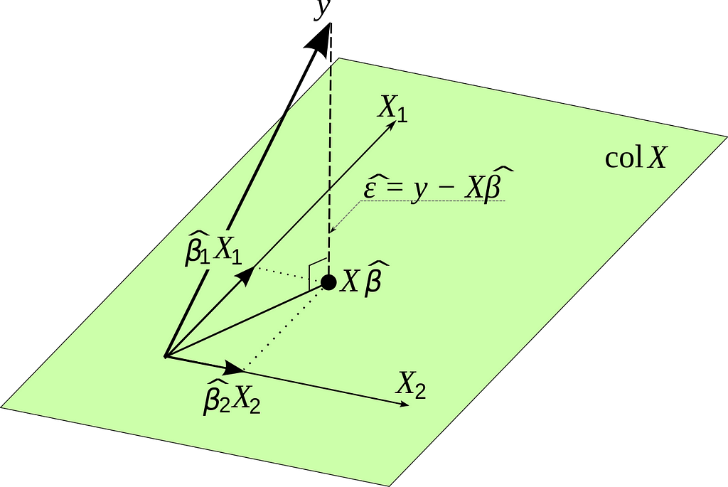
The above image represents a geometric interpretation of Ordinary Least Squares (OLS) or Linear Regression (words used interchangeably in classical statistics). Let’s break down what we’re seeing in an intuitive way:

• Variables (X1 and X2): Imagine you have two variables, X1 and X2. These could represent anything, like the hours you study and the number of practice exams you take, respectively.
• Data Points (y): Now, you have your outcome or what you’re trying to predict, which we call ‘y’. In our example, this could be your score on the actual exam.
• Plane (colX): The plane represents all possible predicted values that you can get by combining different amounts of your variables X1 and X2. In our example, it could represent all possible exam scores you might predict based on different amounts of studying and practice exams.
• Estimated Coefficients (Beta1 and Beta2): These are the best guesses the OLS method makes for how much each variable affects your score. So, Beta 1 might tell you how much your score is predicted to increase for each extra hour of studying, and Beta 2 might tell you how much it increases for each additional practice exam you take.
• Predicted Point (XB^): This is the predicted score you’d get based on the estimated coefficients. It lies on the plane because it’s a combination of your variables X1 and X2 using the estimates from OLS.
• Actual Point (y): This is your actual exam score.
• Error (ε): This is the difference between your actual score and the predicted score. In other words, it’s how off the prediction was from reality.

Now, how does OLS work with all this?

OLS tries to find the values for Beta1 and Beta 2 so that when you predict ‘y’ (the exam score) using X1 and X2 (study hours and practice exams), the error (ε) is as small as possible for all your data points. In the graphic, it’s like adjusting the plane until the vertical dotted lines (which represent errors) are collectively as short as they can be. The shortest distance from the actual data point (y) to the plane (colX) is always a straight line that’s perpendicular to the plane. OLS finds the particular plane where these perpendicular distances are minimized for all points.

In other words, OLS is trying to “fit” the plane as close as possible to your actual scores, while recognizing that it won’t usually pass through all the actual points because real life is rarely that perfect.

It’s like fitting the best sheet of paper beneath a scatter of pencil dots such that the paper is as close as possible to all the dots at the same time.

Let’s go over the main assumptions of OLS and connect them with the visual above:

1. Linearity

Assumption: The relationship between the independent variables (X1, X2) and the dependent variable (y) is linear.

Visual Interpretation: In the image, this is why we use a plane (colX) to represent the combination of X1 and X2. If the relationship were not linear, we wouldn’t be able to represent it with a flat plane; it would be curved or of some other shape.

2. Independence

Assumption: Observations are independent of each other.

Visual Interpretation: Each data point (representing an observation) is plotted independently of the others. If there was dependence, we would see a systematic pattern in the errors (ε), like them all lying on one side of the plane, which would suggest that the way one data point is positioned could predict another, violating this assumption.

3. Homoscedasticity

Assumption: The variance of the error terms (ε) is constant across all levels of the independent variables.

Visual Interpretation: Ideally, the perpendicular distances from the actual data points (y) to the prediction plane (colX) should be uniformly scattered. There shouldn’t be any funnel shape or pattern in these distances; they should look random. If the errors get larger or smaller as X1 or X2 increases, this would violate homoscedasticity.

4. No perfect multicollinearity

Assumption: The independent variables are not perfectly correlated with each other.

Visual Interpretation: In the diagram, X1 and X2 are represented by two arrows pointing in different directions. If they were perfectly correlated, they would point in exactly the same direction, and we would not have a plane but a line. This would make it impossible to estimate the unique effect of X1 and X2 on y.

5. No auto-correlation

Assumption: The error terms are not correlated with each other.

Visual Interpretation: This assumption is about the error terms, which are not explicitly shown in the image, but we infer that each error term (ε) is random and not influenced by the previous or next error term. If there was a pattern (like if one error was always followed by another error of similar size), we would suspect auto-correlation.

6. Exogeneity

Assumption: The error terms have an expected value of zero.

Visual Interpretation: This means that the plane should be positioned such that the errors, on average, cancel each other out. Some data points will be above the plane, and some below, but there’s no systematic bias making them all above or below.

7. Normality of errors (often an assumption for hypothesis testing)

Assumption: The error terms are normally distributed.

Visual Interpretation: While the normality assumption is not something we can visualize in a 3D plot of the data and the model, if we were to look at a histogram of the error terms, we would expect to see the familiar bell curve of a normal distribution.

How does Linear Regression in Machine Learning Universe differ from Ordinary Least Squares based Linear Regression in Classical Statistics?

In classical statistics, Ordinary Least Squares (OLS) can be approached through the lens of Maximum Likelihood Estimation (MLE). Both MLE and OLS aim to find the best parameters for a model, but they come from different philosophies and use different methods to achieve this.

Maximum Likelihood Estimation (MLE) Approach:
MLE is based on probability. It asks the question: “Given a set of data points, what are the most likely parameters of the model that could have generated this data?” MLE assumes a certain probability distribution for the errors (often a normal distribution) and then finds the parameter values that maximize the likelihood of observing the actual data. In the geometric visual, this is akin to adjusting the angle and position of the plane (colX) in such a way that the probability of seeing the actual data points (y) is the highest. The likelihood incorporates not just the distances from the points to the plane (the errors) but also the shape of the error distribution.

Minimization of an Objective Function in Machine Learning (ML):
On the other hand, ML approaches typically frame regression as an optimization problem. The goal is to find the parameters that minimize some objective function, which is usually the sum of squared errors (SSE). This is more of a direct approach than MLE, as it doesn’t make as many assumptions about the underlying probability distribution of the errors. It simply tries to make the distance from the data points to the predicted plane as small as possible, in a squared sense to penalize larger errors more severely. The geometric interpretation is that you’re tilting and moving the plane (colX) to minimize the sum of the squares of the perpendicular distances (the dotted lines) from the actual points (y) to the plane.

Comparing the Two:
Although the procedures differ — one being a probability-based method and the other an optimization technique — they often yield the same result in the case of OLS. This is because when the errors are normally distributed, the MLE for the coefficients of a linear model leads to the same equations as minimizing the sum of squared errors. In the visual, both methods are effectively trying to position the same plane in the space of the variables X1 and X2 such that it best represents the relationship with y.

The main difference is in interpretation and potential generalization. MLE’s framework allows for more flexibility in modeling the error structure and can be extended to models where errors are not assumed to be normally distributed. The ML approach is typically more straightforward and computationally direct, focusing solely on the sum of the squared differences without concerning itself with the underlying probability distribution.

In summary, while MLE and ML minimization approaches might arrive at the same coefficients for an OLS regression, they are conceptually distinct. MLE is probabilistic and rooted in the likelihood of observing the data under a given model, while ML minimization is algorithmic, focusing on the direct reduction of error. The geometric visual remains the same for both, but the rationale behind the position of the plane differs.

Bonus: What happens when you introduce Regularization into the above interpretation?

Regularization is a technique used to prevent overfitting in models, which can occur when a model is too complex and starts to capture the noise in the data rather than just the true underlying pattern. There are different types of regularization, but the two most common are:

• Lasso Regression (L1 regularization): This adds a penalty equal to the absolute value of the magnitude of coefficients. It can reduce some coefficients to zero, effectively performing feature selection.
• Ridge Regression (L2 regularization): This adds a penalty equal to the square of the magnitude of coefficients. All coefficients are shrunk by the same factor and none are zeroed out.

Let’s use the example of fitting a blanket (representing our regression model) over a bed (representing our data). In OLS without regularization, we are trying to fit the blanket so that it touches as many points (data points) on the bed as possible, minimizing the distance between the blanket and the bed’s surface (the errors).

Now, imagine if the bed is quite bumpy and our blanket is very flexible. Without regularization, we might fit the blanket so snugly that it fits every single bump and dip, even the small ones that are just due to someone not smoothing out the bedspread — this is overfitting.

Introducing Regularization:

• With Lasso (L1): It’s like saying, “I want the blanket to fit well, but I also want it to be smooth with as few folds as possible.” Each fold represents a feature in our model, and L1 regularization tries to minimize the number of folds. In the end, you’ll have a blanket that fits the bed well but might not get into every nook and cranny, especially if those are just noise. In the geometric visual, Lasso would try to keep the plane (colX) well-fitted to the points but might flatten out in the direction of less important variables (shrinking coefficients to zero).
• With Ridge (L2): This is like wanting a snug fit but also wanting the blanket to be evenly spread out without any part being too far from the bed. So even though the blanket still fits the bed closely, it won’t get overly contorted to fit the minor bumps. In the geometric visual, Ridge adds a penalty that constrains the coefficients, shrinking them towards zero but not exactly to zero. This keeps the plane close to the points but prevents it from tilting too sharply to fit any particular points too closely, thus maintaining a bit of a distance (bias) to prevent overfitting to the noise.

Visual Interpretation with Regularization:
When regularization is added to the geometrical interpretation:

• The plane (colX) may no longer pass as close to each individual data point (y) as it did before. Regularization introduces a bit of bias on purpose.
• The plane will tend to be more stable and less tilted towards any individual outlier points, as the penalty for having large coefficients means the model can’t be too sensitive to any single data point or feature.
• The length of the vectors (Beta1X1 and Beta2X2) might be shorter, reflecting the fact that the influence of each variable on the prediction is being deliberately restrained.

In essence, regularization trades off a little bit of the model’s ability to fit the training data perfectly in return for improved model generalization, which means it will perform better on unseen data, not just the data it was trained on. It’s like choosing a slightly looser blanket fit that’s good enough for all practical purposes, rather than one that fits every single contour but might be impractical or too specific to just one bed.

Conclusion

In summary, the geometric interpretation of linear regression bridges the gap between classical statistics and machine learning, offering an intuitive understanding of this fundamental technique. While classical statistics approach linear regression through Ordinary Least Squares and machine learning often employs Maximum Likelihood Estimation or objective function minimization, both methods ultimately seek to minimize prediction error in a visually comprehensible way.

The introduction of regularization techniques like Lasso and Ridge further enriches this interpretation, highlighting the balance between model accuracy and generalizability. These methods prevent overfitting, ensuring that the model remains robust and effective for new, unseen data.

Overall, this geometric perspective not only demystifies linear regression but also underscores the importance of foundational concepts in the evolving landscape of data analysis and machine learning. It’s a powerful reminder of how complex algorithms can be rooted in simple, yet profound, geometric principles.

Geometrical Interpretation of Linear Regression in Machine Learning versus Classical Statistics was originally published in Towards Data Science on Medium, where people are continuing the conversation by highlighting and responding to this story.

Demystifying the confusion about Linear Regression Visually and Analytically

The above image represents a geometric interpretation of Ordinary Least Squares (OLS) or Linear Regression (words used interchangeably in classical statistics). Let’s break down what we’re seeing in an intuitive way:

• Variables (X1 and X2): Imagine you have two variables, X1 and X2. These could represent anything, like the hours you study and the number of practice exams you take, respectively.
• Data Points (y): Now, you have your outcome or what you’re trying to predict, which we call ‘y’. In our example, this could be your score on the actual exam.
• Plane (colX): The plane represents all possible predicted values that you can get by combining different amounts of your variables X1 and X2. In our example, it could represent all possible exam scores you might predict based on different amounts of studying and practice exams.
• Estimated Coefficients (Beta1 and Beta2): These are the best guesses the OLS method makes for how much each variable affects your score. So, Beta 1 might tell you how much your score is predicted to increase for each extra hour of studying, and Beta 2 might tell you how much it increases for each additional practice exam you take.
• Predicted Point (XB^): This is the predicted score you’d get based on the estimated coefficients. It lies on the plane because it’s a combination of your variables X1 and X2 using the estimates from OLS.
• Actual Point (y): This is your actual exam score.
• Error (ε): This is the difference between your actual score and the predicted score. In other words, it’s how off the prediction was from reality.

Now, how does OLS work with all this?

OLS tries to find the values for Beta1 and Beta 2 so that when you predict ‘y’ (the exam score) using X1 and X2 (study hours and practice exams), the error (ε) is as small as possible for all your data points. In the graphic, it’s like adjusting the plane until the vertical dotted lines (which represent errors) are collectively as short as they can be. The shortest distance from the actual data point (y) to the plane (colX) is always a straight line that’s perpendicular to the plane. OLS finds the particular plane where these perpendicular distances are minimized for all points.

In other words, OLS is trying to “fit” the plane as close as possible to your actual scores, while recognizing that it won’t usually pass through all the actual points because real life is rarely that perfect.

It’s like fitting the best sheet of paper beneath a scatter of pencil dots such that the paper is as close as possible to all the dots at the same time.

Let’s go over the main assumptions of OLS and connect them with the visual above:

1. Linearity

Assumption: The relationship between the independent variables (X1, X2) and the dependent variable (y) is linear.

Visual Interpretation: In the image, this is why we use a plane (colX) to represent the combination of X1 and X2. If the relationship were not linear, we wouldn’t be able to represent it with a flat plane; it would be curved or of some other shape.

2. Independence

Assumption: Observations are independent of each other.

Visual Interpretation: Each data point (representing an observation) is plotted independently of the others. If there was dependence, we would see a systematic pattern in the errors (ε), like them all lying on one side of the plane, which would suggest that the way one data point is positioned could predict another, violating this assumption.

3. Homoscedasticity

Assumption: The variance of the error terms (ε) is constant across all levels of the independent variables.

Visual Interpretation: Ideally, the perpendicular distances from the actual data points (y) to the prediction plane (colX) should be uniformly scattered. There shouldn’t be any funnel shape or pattern in these distances; they should look random. If the errors get larger or smaller as X1 or X2 increases, this would violate homoscedasticity.

4. No perfect multicollinearity

Assumption: The independent variables are not perfectly correlated with each other.

Visual Interpretation: In the diagram, X1 and X2 are represented by two arrows pointing in different directions. If they were perfectly correlated, they would point in exactly the same direction, and we would not have a plane but a line. This would make it impossible to estimate the unique effect of X1 and X2 on y.

5. No auto-correlation

Assumption: The error terms are not correlated with each other.

Visual Interpretation: This assumption is about the error terms, which are not explicitly shown in the image, but we infer that each error term (ε) is random and not influenced by the previous or next error term. If there was a pattern (like if one error was always followed by another error of similar size), we would suspect auto-correlation.

6. Exogeneity

Assumption: The error terms have an expected value of zero.

Visual Interpretation: This means that the plane should be positioned such that the errors, on average, cancel each other out. Some data points will be above the plane, and some below, but there’s no systematic bias making them all above or below.

7. Normality of errors (often an assumption for hypothesis testing)

Assumption: The error terms are normally distributed.

Visual Interpretation: While the normality assumption is not something we can visualize in a 3D plot of the data and the model, if we were to look at a histogram of the error terms, we would expect to see the familiar bell curve of a normal distribution.

How does Linear Regression in Machine Learning Universe differ from Ordinary Least Squares based Linear Regression in Classical Statistics?

In classical statistics, Ordinary Least Squares (OLS) can be approached through the lens of Maximum Likelihood Estimation (MLE). Both MLE and OLS aim to find the best parameters for a model, but they come from different philosophies and use different methods to achieve this.

Maximum Likelihood Estimation (MLE) Approach:
MLE is based on probability. It asks the question: “Given a set of data points, what are the most likely parameters of the model that could have generated this data?” MLE assumes a certain probability distribution for the errors (often a normal distribution) and then finds the parameter values that maximize the likelihood of observing the actual data. In the geometric visual, this is akin to adjusting the angle and position of the plane (colX) in such a way that the probability of seeing the actual data points (y) is the highest. The likelihood incorporates not just the distances from the points to the plane (the errors) but also the shape of the error distribution.

Minimization of an Objective Function in Machine Learning (ML):
On the other hand, ML approaches typically frame regression as an optimization problem. The goal is to find the parameters that minimize some objective function, which is usually the sum of squared errors (SSE). This is more of a direct approach than MLE, as it doesn’t make as many assumptions about the underlying probability distribution of the errors. It simply tries to make the distance from the data points to the predicted plane as small as possible, in a squared sense to penalize larger errors more severely. The geometric interpretation is that you’re tilting and moving the plane (colX) to minimize the sum of the squares of the perpendicular distances (the dotted lines) from the actual points (y) to the plane.

Comparing the Two:
Although the procedures differ — one being a probability-based method and the other an optimization technique — they often yield the same result in the case of OLS. This is because when the errors are normally distributed, the MLE for the coefficients of a linear model leads to the same equations as minimizing the sum of squared errors. In the visual, both methods are effectively trying to position the same plane in the space of the variables X1 and X2 such that it best represents the relationship with y.

The main difference is in interpretation and potential generalization. MLE’s framework allows for more flexibility in modeling the error structure and can be extended to models where errors are not assumed to be normally distributed. The ML approach is typically more straightforward and computationally direct, focusing solely on the sum of the squared differences without concerning itself with the underlying probability distribution.

In summary, while MLE and ML minimization approaches might arrive at the same coefficients for an OLS regression, they are conceptually distinct. MLE is probabilistic and rooted in the likelihood of observing the data under a given model, while ML minimization is algorithmic, focusing on the direct reduction of error. The geometric visual remains the same for both, but the rationale behind the position of the plane differs.

Bonus: What happens when you introduce Regularization into the above interpretation?

Regularization is a technique used to prevent overfitting in models, which can occur when a model is too complex and starts to capture the noise in the data rather than just the true underlying pattern. There are different types of regularization, but the two most common are:

• Lasso Regression (L1 regularization): This adds a penalty equal to the absolute value of the magnitude of coefficients. It can reduce some coefficients to zero, effectively performing feature selection.
• Ridge Regression (L2 regularization): This adds a penalty equal to the square of the magnitude of coefficients. All coefficients are shrunk by the same factor and none are zeroed out.

Let’s use the example of fitting a blanket (representing our regression model) over a bed (representing our data). In OLS without regularization, we are trying to fit the blanket so that it touches as many points (data points) on the bed as possible, minimizing the distance between the blanket and the bed’s surface (the errors).

Now, imagine if the bed is quite bumpy and our blanket is very flexible. Without regularization, we might fit the blanket so snugly that it fits every single bump and dip, even the small ones that are just due to someone not smoothing out the bedspread — this is overfitting.

Introducing Regularization:

• With Lasso (L1): It’s like saying, “I want the blanket to fit well, but I also want it to be smooth with as few folds as possible.” Each fold represents a feature in our model, and L1 regularization tries to minimize the number of folds. In the end, you’ll have a blanket that fits the bed well but might not get into every nook and cranny, especially if those are just noise. In the geometric visual, Lasso would try to keep the plane (colX) well-fitted to the points but might flatten out in the direction of less important variables (shrinking coefficients to zero).
• With Ridge (L2): This is like wanting a snug fit but also wanting the blanket to be evenly spread out without any part being too far from the bed. So even though the blanket still fits the bed closely, it won’t get overly contorted to fit the minor bumps. In the geometric visual, Ridge adds a penalty that constrains the coefficients, shrinking them towards zero but not exactly to zero. This keeps the plane close to the points but prevents it from tilting too sharply to fit any particular points too closely, thus maintaining a bit of a distance (bias) to prevent overfitting to the noise.

Visual Interpretation with Regularization:
When regularization is added to the geometrical interpretation:

• The plane (colX) may no longer pass as close to each individual data point (y) as it did before. Regularization introduces a bit of bias on purpose.
• The plane will tend to be more stable and less tilted towards any individual outlier points, as the penalty for having large coefficients means the model can’t be too sensitive to any single data point or feature.
• The length of the vectors (Beta1X1 and Beta2X2) might be shorter, reflecting the fact that the influence of each variable on the prediction is being deliberately restrained.

In essence, regularization trades off a little bit of the model’s ability to fit the training data perfectly in return for improved model generalization, which means it will perform better on unseen data, not just the data it was trained on. It’s like choosing a slightly looser blanket fit that’s good enough for all practical purposes, rather than one that fits every single contour but might be impractical or too specific to just one bed.

Conclusion

In summary, the geometric interpretation of linear regression bridges the gap between classical statistics and machine learning, offering an intuitive understanding of this fundamental technique. While classical statistics approach linear regression through Ordinary Least Squares and machine learning often employs Maximum Likelihood Estimation or objective function minimization, both methods ultimately seek to minimize prediction error in a visually comprehensible way.

The introduction of regularization techniques like Lasso and Ridge further enriches this interpretation, highlighting the balance between model accuracy and generalizability. These methods prevent overfitting, ensuring that the model remains robust and effective for new, unseen data.

Overall, this geometric perspective not only demystifies linear regression but also underscores the importance of foundational concepts in the evolving landscape of data analysis and machine learning. It’s a powerful reminder of how complex algorithms can be rooted in simple, yet profound, geometric principles.

Geometrical Interpretation of Linear Regression in Machine Learning versus Classical Statistics was originally published in Towards Data Science on Medium, where people are continuing the conversation by highlighting and responding to this story.

FOLLOW US ON GOOGLE NEWS

Read original article here