
How to Simplify Hypothesis Testing for Linear Regression in Python | by Andreas Martinson | Jul, 2022
Statistics
What is homoscedasticity again?
I find myself coming back to the basics to refresh my statistical knowledge over and over again. Most people’s first introduction to statistics begins by learning hypothesis testing, which is followed soon after by t-tests and linear regression. This article is a refresher of how to use linear regression for hypothesis testing along with the assumptions that have to be satisfied in order to trust the results of your linear regression statistical test. I also want to share a Python function I made to quickly check the 5 statistical assumptions that need to be satisfied for hypothesis testing using linear regression.
A Quick Reminder Regarding Linear Regression
Before I share the 4 assumptions that should be met in order to run a linear regression hypothesis test, there is one important point to keep in mind regarding linear regression. Linear regression can be thought of as a dual purpose tool:
- To predict future values for the y variable
- To infer if the trend is statistically significant
This is important to remember because it means that your data does not have to meet the requirements for a linear regression hypothesis test if you are using the regression to predict future values. You need to meet the hypothesis test assumptions if you are trying to determine if there is an actual trend (aka the trend is statistically significant).
Linear Regression and Machine Learning
When compared to machine learning, traditional statistics is more associated with inference of signals in the data; whereas machine learning is more focused on prediction. Of all the models there are to choose from for machine learning, linear regression is one of the simplest models you can use and is typically used as a benchmark when building new machine learning models based on continuous data (a logistic regression would be the equivalent if you are working with categorical data). You can see why both statistics and machine learning are necessary tools as a data professional. A good reminder to remember is that statistics leans more towards inference and machine learning towards prediction. That being said, it’s also worth noting that statistics provided the bedrock for machine learning to be created in the first place.
Why the Linear Regression Hypothesis Test is Important
Hypothesis testing helps us to determine if there is enough signal in our data to be confident that we can reject the null hypothesis. Essentially, it answers the question, “Can I be confident in the patterns that I’m seeing in the data or is what I am seeing just noise?” We use statistics to infer relationships and meaning that exist in the data.
Now in order to make inferences from our data using a linear regression hypothesis test, we need to determine what we are testing. In order to explain that, I need to share this simple formula:
y = mx + b
I think most people who have had high school math will remember that this is the equation for the slope of a line.
The more formal representation of this formula in terms of linear regression is:
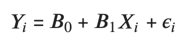
Where B0 is the intercept and B1 is the slope. X and Y represent the independent and dependent variables respectively and epsilon is the error term.
A linear regression hypothesis test for the slope of a line (B1) looks like the following:
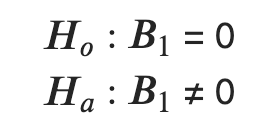
These mathematical notations state that the null hypothesis (Ho) is that the slope (B1) is equal to 0 (i.e. the slope is flat). The alternative hypothesis (Ha) is that the slope is not equal to 0.
Side note: There is another hypothesis test that is more seldom used with linear regression, which is a hypothesis regarding the intercept. It’s used less since we’re typically concerned with the slope of the line.
The 4 Assumptions for Linear Regression Hypothesis Testing
- There is a linear regression relation between Y and X
- The error terms (residuals) are normally distributed
- The variance of the error terms is constant over all X values (homeoscadiscticity)
- The error terms are independent
In order to demonstrate testing these statistical assumptions for linear regression we need a dataset. I’ll be using the cars dataset from the R standard library. The dataset is really simple and looks like this:
pip install rdatasets
from rdatasets import data as rdatadat = rdata("cars")
dat
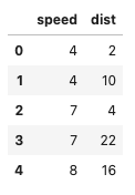
We will be predicting the distance that a 1920’s car will go before stopping given a specific speed.
Let’s first create the linear regression model and then go through the steps of checking assumptions.
Side note: There is technically a 5th assumption that the X values are fixed and measured without error. However, that assumption is not something you would create a diagnostic plot for and so it has been omitted.
Creating the Linear Regression Diagnostic Plots In R and Python
I typically code in Python, but I want to show how to create the linear regression model in both R and Python to demonstrate how easy it is to check the statistical assumptions in R.
Linear Regression in R
cars.lm <- lm(dist ~ speed, data=cars)
Then to check assumptions all that you need to do is call the plot function and select the first two plots
plot(cars.lm, which=1:2)
This gives you the following graphs:
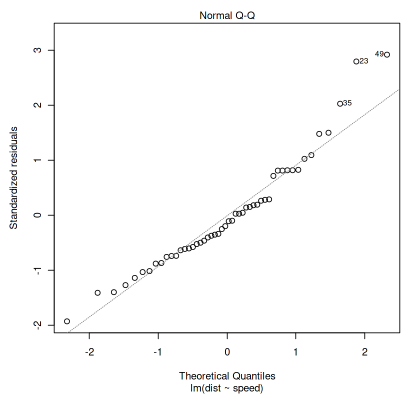
The first is the residual vs. fitted graph and the second is the QQ plot. I will explain these two plots in more detail below.
These two plots are almost all that you need to test the 4 assumptions above. There doesn’t seem to be as quick and easy of a way to check linear regression assumptions in Python as in R so I made a quick function to do the same thing.
Linear Regression in Python
This is how you would run a linear regression for the same cars dataset in Python:
from statsmodels.formula.api import ols
from rdatasets import data as rdatacars = rdata("cars")
cars_lm = ols("dist ~ speed", data=cars).fit()
Side Note: Linear regression in R is part of the built in function, whereas in Python I am using the statsmodels package.
However, to get the same two diagnostic plots above, you would have to run the following commands separately.
QQ Plot in Python
import statsmodels.api as sm
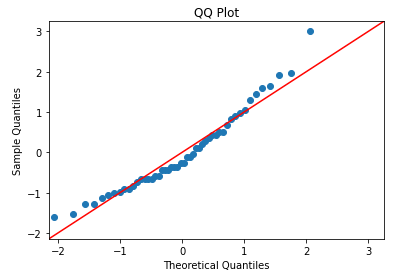
import matplotlib.pyplot as pltsm.qqplot(cars['dist'], line='45', fit=True)
plt.title('QQ Plot')
plt.show()
Residuals vs Fitted in Python
from statsmodels.formula.api import ols
import statsmodels.api as sm
from rdatasets import data as rdata
import matplotlib.pyplot as plt# Import Data
cars = rdata("cars")# Fit the model
cars_lm = ols("dist ~ speed", data=cars).fit()# Find the residuals
residuals = cars['dist'] - cars_lm.predict()# Get the smoothed lowess line
lowess = sm.nonparametric.lowess
lowess_values = pd.Series(lowess(residuals, cars['speed'])[:,1])# Plot the fitted v residuals graph
plt.scatter(cars['speed'], residuals)
plt.plot(cars['speed'], lowess_values, c='r')
plt.axhline(y=0, c='black', alpha=.75)
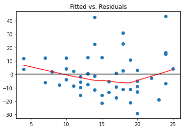
plt.title('Fitted vs. Residuals')
plt.show()
A Simplified Python Function for Linear Regression Diagnostic Plots
The effort required to create the plots above isn’t too terrible, but it’s still more than I want to have to type in every time I am checking linear regression assumptions. There’s also some more diagnostic plots that I would like to have, such as a histogram for checking normal distributions in addition to the QQ Plot. I would also like another plot to check assumption #4, which was that the error terms are independent.
So I made a Python function in order to quickly check the OLS assumptions. I will refer back to this function in the future and I hope that you find it useful as well. I included the gist below, but the function is saved in this git repo here. Suggestions for improvement are welcome.
As a side note, I found another blog post about creating R diagnostic plots in Python here
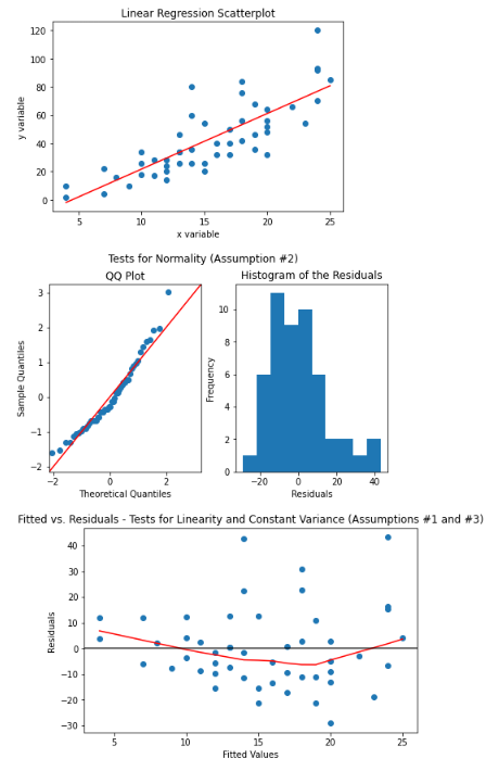
If I pass the cars dataset into the check_ols_assumption function, I will get the following diagnostic plot output:
cars = rdata("cars")
cars_lm = ols("dist ~ speed", data=dat).fit()check_ols_assumptions(cars['speed'], cars['dist'], cars_lm.predict())
Linear Regression Hypothesis Testing Assumptions Explained
Now that I’ve shared the function I created for quick linear regression hypothesis testing in Python, I want to give a quick refresher on how to interpret the diagnostic plots and how the diagnostic plots help determine if the linear regression assumptions are satisfied.
- Linear Relationship
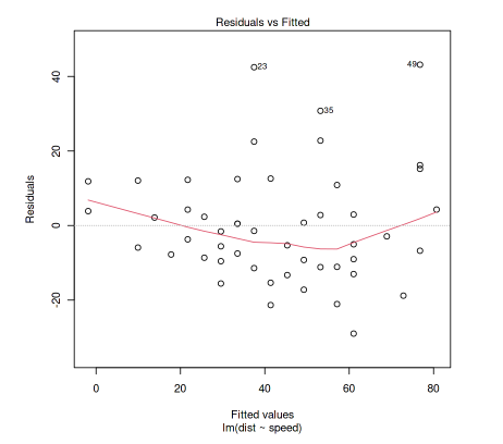
The diagnostic plot to determine linearity is the fitted v. residuals plot:
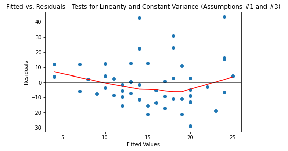
The fitted values on the X-axis are the values predicted from the linear regression. On the Y-axis are the residuals, which are the difference between the predicted (fitted) values and the actual Y values.
The linear relation is assumed to be satisfied if there are no apparent trends in the plot. The above plot satisfies this assumption. Here is an example of a diagnostic plot that fails this assumption:
# Create a synthetic dataset
np.random.seed(42)
x_var = np.arange(0,10,.1)
y_var = np.sin(x_var)data = pd.DataFrame({'x_var':x_var, 'y_var':y_var})ols_result = ols("y_var ~ x_var", data=data).fit()
check_ols_assumptions(data['x_var'], data['y_var'], ols_result.predict())
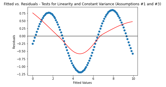
This graph shows the residuals of a linear regression model for a sin function. Since there is an obvious trend (shown by the scatter plot values as well as the red line from the lowess regression), it fails the assumption that the relationship between X and Y are linear.
Side note: For more information about lowess regression, check out this article here
2. The Error Terms are Normally Distributed
The key point to remember with this assumption is that the X or Y variables do not have to be normally distributed, it’s the error terms or residuals that need to be. Another important point to remember is just because a plot is linear, doesn’t mean the distribution can be considered normal.
Here is the diagnostic plot for checking that the error terms (residuals) are normally distributed:
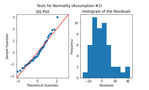
I use both the QQ plot and histogram to check for normality. This assumption is satisfied if the QQ plot points roughly line up with the 45 degree line. Another way to check would be the histogram, the residuals can be considered normal if the distribution follows a normal (gaussian) bell curve. To learn more about QQ plots, please refer to this article here.
3. The Variance of the Error Terms is Constant Over All X Values
The fitted vs residuals plot is used again to determine if the variance is constant. Here is the plot again for reference:
The constant variance assumption is assumed to be satisfied if the vertical spread of the residuals remains roughly consistent across all fitted values. The cars dataset looks like it might be questionably passing this assumption. Here is a more clear example of a dataset that would fail this assumption:
# Create a synthetic dataset
np.random.seed(42)
x_var = np.arange(0,10,.1)
y_var = np.random.normal(0,.1,100) * x_vardata = pd.DataFrame({'x_var':x_var, 'y_var':y_var})ols_result = ols("y_var ~ x_var", data=data).fit()
check_ols_assumptions(data['x_var'], data['y_var'], ols_result.predict())
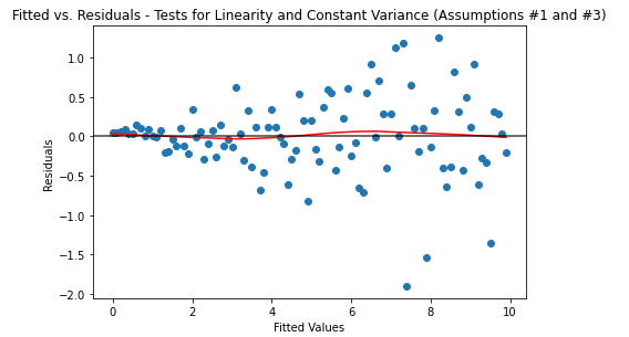
This example shows hows the data starts spreading further with increasing values of X. This violates this assumption since the data is spreading further and further apart with higher values of X .
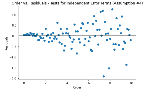
4. The Error Terms are Independent
This assumption can only be checked if you know the order that the data was collected. Most often, this can be checked when there is a time component in your dataset (but by using a time column, you assume the time the data was collected was at the same time as that column). If there is a trend in the residual values over time, then this assumption is violated.
If the values were already in the correct order, it will look the same as the fitted vs. residuals plot. There is a default parameter in the check_ols_assumptions above where the time variable can be passed if it exists in your dataset.
Conclusion
There you have it, a quick refresher on using a linear regression for statistical analysis. I hope you will find the check_ols_assumptions function useful, please let me know if you have any feedback 😄
Statistics
What is homoscedasticity again?

I find myself coming back to the basics to refresh my statistical knowledge over and over again. Most people’s first introduction to statistics begins by learning hypothesis testing, which is followed soon after by t-tests and linear regression. This article is a refresher of how to use linear regression for hypothesis testing along with the assumptions that have to be satisfied in order to trust the results of your linear regression statistical test. I also want to share a Python function I made to quickly check the 5 statistical assumptions that need to be satisfied for hypothesis testing using linear regression.
A Quick Reminder Regarding Linear Regression
Before I share the 4 assumptions that should be met in order to run a linear regression hypothesis test, there is one important point to keep in mind regarding linear regression. Linear regression can be thought of as a dual purpose tool:
- To predict future values for the y variable
- To infer if the trend is statistically significant
This is important to remember because it means that your data does not have to meet the requirements for a linear regression hypothesis test if you are using the regression to predict future values. You need to meet the hypothesis test assumptions if you are trying to determine if there is an actual trend (aka the trend is statistically significant).
Linear Regression and Machine Learning
When compared to machine learning, traditional statistics is more associated with inference of signals in the data; whereas machine learning is more focused on prediction. Of all the models there are to choose from for machine learning, linear regression is one of the simplest models you can use and is typically used as a benchmark when building new machine learning models based on continuous data (a logistic regression would be the equivalent if you are working with categorical data). You can see why both statistics and machine learning are necessary tools as a data professional. A good reminder to remember is that statistics leans more towards inference and machine learning towards prediction. That being said, it’s also worth noting that statistics provided the bedrock for machine learning to be created in the first place.
Why the Linear Regression Hypothesis Test is Important
Hypothesis testing helps us to determine if there is enough signal in our data to be confident that we can reject the null hypothesis. Essentially, it answers the question, “Can I be confident in the patterns that I’m seeing in the data or is what I am seeing just noise?” We use statistics to infer relationships and meaning that exist in the data.
Now in order to make inferences from our data using a linear regression hypothesis test, we need to determine what we are testing. In order to explain that, I need to share this simple formula:
y = mx + b
I think most people who have had high school math will remember that this is the equation for the slope of a line.
The more formal representation of this formula in terms of linear regression is:
Where B0 is the intercept and B1 is the slope. X and Y represent the independent and dependent variables respectively and epsilon is the error term.
A linear regression hypothesis test for the slope of a line (B1) looks like the following:
These mathematical notations state that the null hypothesis (Ho) is that the slope (B1) is equal to 0 (i.e. the slope is flat). The alternative hypothesis (Ha) is that the slope is not equal to 0.
Side note: There is another hypothesis test that is more seldom used with linear regression, which is a hypothesis regarding the intercept. It’s used less since we’re typically concerned with the slope of the line.
The 4 Assumptions for Linear Regression Hypothesis Testing
- There is a linear regression relation between Y and X
- The error terms (residuals) are normally distributed
- The variance of the error terms is constant over all X values (homeoscadiscticity)
- The error terms are independent
In order to demonstrate testing these statistical assumptions for linear regression we need a dataset. I’ll be using the cars dataset from the R standard library. The dataset is really simple and looks like this:
pip install rdatasets
from rdatasets import data as rdatadat = rdata("cars")
dat
We will be predicting the distance that a 1920’s car will go before stopping given a specific speed.
Let’s first create the linear regression model and then go through the steps of checking assumptions.
Side note: There is technically a 5th assumption that the X values are fixed and measured without error. However, that assumption is not something you would create a diagnostic plot for and so it has been omitted.
Creating the Linear Regression Diagnostic Plots In R and Python
I typically code in Python, but I want to show how to create the linear regression model in both R and Python to demonstrate how easy it is to check the statistical assumptions in R.
Linear Regression in R
cars.lm <- lm(dist ~ speed, data=cars)
Then to check assumptions all that you need to do is call the plot function and select the first two plots
plot(cars.lm, which=1:2)
This gives you the following graphs:
The first is the residual vs. fitted graph and the second is the QQ plot. I will explain these two plots in more detail below.
These two plots are almost all that you need to test the 4 assumptions above. There doesn’t seem to be as quick and easy of a way to check linear regression assumptions in Python as in R so I made a quick function to do the same thing.
Linear Regression in Python
This is how you would run a linear regression for the same cars dataset in Python:
from statsmodels.formula.api import ols
from rdatasets import data as rdatacars = rdata("cars")
cars_lm = ols("dist ~ speed", data=cars).fit()
Side Note: Linear regression in R is part of the built in function, whereas in Python I am using the statsmodels package.
However, to get the same two diagnostic plots above, you would have to run the following commands separately.
QQ Plot in Python
import statsmodels.api as sm
import matplotlib.pyplot as pltsm.qqplot(cars['dist'], line='45', fit=True)
plt.title('QQ Plot')
plt.show()
Residuals vs Fitted in Python
from statsmodels.formula.api import ols
import statsmodels.api as sm
from rdatasets import data as rdata
import matplotlib.pyplot as plt# Import Data
cars = rdata("cars")# Fit the model
cars_lm = ols("dist ~ speed", data=cars).fit()# Find the residuals
residuals = cars['dist'] - cars_lm.predict()# Get the smoothed lowess line
lowess = sm.nonparametric.lowess
lowess_values = pd.Series(lowess(residuals, cars['speed'])[:,1])# Plot the fitted v residuals graph
plt.scatter(cars['speed'], residuals)
plt.plot(cars['speed'], lowess_values, c='r')
plt.axhline(y=0, c='black', alpha=.75)
plt.title('Fitted vs. Residuals')
plt.show()
A Simplified Python Function for Linear Regression Diagnostic Plots
The effort required to create the plots above isn’t too terrible, but it’s still more than I want to have to type in every time I am checking linear regression assumptions. There’s also some more diagnostic plots that I would like to have, such as a histogram for checking normal distributions in addition to the QQ Plot. I would also like another plot to check assumption #4, which was that the error terms are independent.
So I made a Python function in order to quickly check the OLS assumptions. I will refer back to this function in the future and I hope that you find it useful as well. I included the gist below, but the function is saved in this git repo here. Suggestions for improvement are welcome.
As a side note, I found another blog post about creating R diagnostic plots in Python here
If I pass the cars dataset into the check_ols_assumption function, I will get the following diagnostic plot output:
cars = rdata("cars")
cars_lm = ols("dist ~ speed", data=dat).fit()check_ols_assumptions(cars['speed'], cars['dist'], cars_lm.predict())
Linear Regression Hypothesis Testing Assumptions Explained
Now that I’ve shared the function I created for quick linear regression hypothesis testing in Python, I want to give a quick refresher on how to interpret the diagnostic plots and how the diagnostic plots help determine if the linear regression assumptions are satisfied.
- Linear Relationship
The diagnostic plot to determine linearity is the fitted v. residuals plot:
The fitted values on the X-axis are the values predicted from the linear regression. On the Y-axis are the residuals, which are the difference between the predicted (fitted) values and the actual Y values.
The linear relation is assumed to be satisfied if there are no apparent trends in the plot. The above plot satisfies this assumption. Here is an example of a diagnostic plot that fails this assumption:
# Create a synthetic dataset
np.random.seed(42)
x_var = np.arange(0,10,.1)
y_var = np.sin(x_var)data = pd.DataFrame({'x_var':x_var, 'y_var':y_var})ols_result = ols("y_var ~ x_var", data=data).fit()
check_ols_assumptions(data['x_var'], data['y_var'], ols_result.predict())
This graph shows the residuals of a linear regression model for a sin function. Since there is an obvious trend (shown by the scatter plot values as well as the red line from the lowess regression), it fails the assumption that the relationship between X and Y are linear.
Side note: For more information about lowess regression, check out this article here
2. The Error Terms are Normally Distributed
The key point to remember with this assumption is that the X or Y variables do not have to be normally distributed, it’s the error terms or residuals that need to be. Another important point to remember is just because a plot is linear, doesn’t mean the distribution can be considered normal.
Here is the diagnostic plot for checking that the error terms (residuals) are normally distributed:
I use both the QQ plot and histogram to check for normality. This assumption is satisfied if the QQ plot points roughly line up with the 45 degree line. Another way to check would be the histogram, the residuals can be considered normal if the distribution follows a normal (gaussian) bell curve. To learn more about QQ plots, please refer to this article here.
3. The Variance of the Error Terms is Constant Over All X Values
The fitted vs residuals plot is used again to determine if the variance is constant. Here is the plot again for reference:
The constant variance assumption is assumed to be satisfied if the vertical spread of the residuals remains roughly consistent across all fitted values. The cars dataset looks like it might be questionably passing this assumption. Here is a more clear example of a dataset that would fail this assumption:
# Create a synthetic dataset
np.random.seed(42)
x_var = np.arange(0,10,.1)
y_var = np.random.normal(0,.1,100) * x_vardata = pd.DataFrame({'x_var':x_var, 'y_var':y_var})ols_result = ols("y_var ~ x_var", data=data).fit()
check_ols_assumptions(data['x_var'], data['y_var'], ols_result.predict())
This example shows hows the data starts spreading further with increasing values of X. This violates this assumption since the data is spreading further and further apart with higher values of X .
4. The Error Terms are Independent
This assumption can only be checked if you know the order that the data was collected. Most often, this can be checked when there is a time component in your dataset (but by using a time column, you assume the time the data was collected was at the same time as that column). If there is a trend in the residual values over time, then this assumption is violated.
If the values were already in the correct order, it will look the same as the fitted vs. residuals plot. There is a default parameter in the check_ols_assumptions above where the time variable can be passed if it exists in your dataset.
Conclusion
There you have it, a quick refresher on using a linear regression for statistical analysis. I hope you will find the check_ols_assumptions function useful, please let me know if you have any feedback 😄
Denial of responsibility! Techno Blender is an automatic aggregator of the all world’s media. In each content, the hyperlink to the primary source is specified. All trademarks belong to their rightful owners, all materials to their authors. If you are the owner of the content and do not want us to publish your materials, please contact us by email – [email protected]. The content will be deleted within 24 hours.