Linear Regression with OLS: Heteroskedasticity and Autocorrelation | by Aaron Zhu | Jun, 2022

Understand OLS Linear Regression with a bit of math

Heteroskedasticity and Autocorrelation are unavoidable issues we need to address when setting up a linear regression. In this article, let’s dive deeper into what are Heteroskedasticity and Autocorrelation, what are the Consequences, and remedies to handle issues.

A typical linear regression takes the form as follows. The response variable (i.e., Y) is explained as a linear combination of explanatory variables (e.g., the intercept, X1, X2, X3, …) and ε is the error term (i.e., a random variable) that represents the difference between the fitted response value and the actual response value.

Homoscedasticity

Under the assumption of Homoscedasticity, the error term should have constant variance and iid. In other words, the diagonal values in the variance-covariance matrix of the error term should be constant and off-diagonal values should be all 0.

Heteroskedasticity

In the real world, Homoscedasticity assumption may not be plausible. The variance of the error terms may not remain the same. Sometimes the variance of the error terms depends on the explanatory variable in the model.

For example, the number of bedrooms is usually used to predict house prices, we see that the prediction error is larger for houses with 6+ bedrooms than the ones with 2 bedrooms because houses with 6+ bedrooms are typically worth a lot more than 2-bedroom houses, therefore, have larger unexplained and sometimes irreducible price variance, which leaks into the error term.

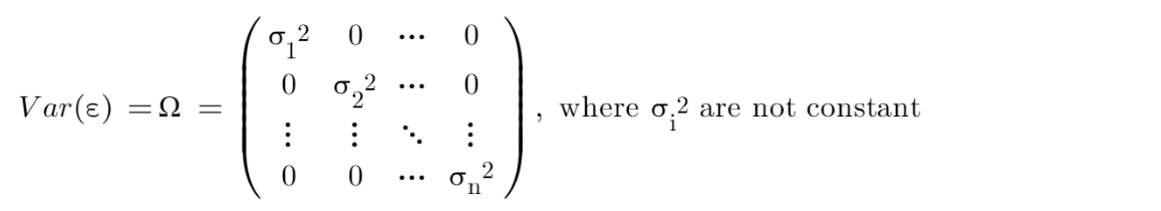
We call the error term whose variances are NOT constant across observations Heteroskedastic error. This property is called Heteroskedasticity.

Autocorrelation

When there is autocorrelation in the model, the error terms are correlated. It means off-diagonal values of the covariance matrix of error terms are NOT all 0s.

There are some possible sources of autocorrelation. In the time-series data, time is the factor that produces autocorrelation. For example, the current stock price is influenced by the prices from previous trading days (e.g., the stock price is more likely to fall after a huge price hike). In the cross-section data, the neighboring units tend to have similar characteristics.

Remedy 1: Heteroskedasticity-consistent (HC) and Heteroskedasticity- Autocorrelation-consistent (HAC) Standard Errors

Under Heteroskedasticity or Autocorrelation, we can still use the inefficient OLS estimator, but many literatures suggest using Heteroskedasticity-consistent (HC) standard errors (aka, robust standard errors, White standard errors) or Heteroskedasticity- Autocorrelation-consistent (HAC) Standard Errors (aka, Newey-West Standard Error) that allow for the presence of Heteroskedasticity or Autocorrelation. These are the easiest and most common solutions.

Many econometricians argue that one should always use robust standard errors because one never can rely on Homoskedasticity.

Remedy 2: Generalized Least Square (GLS) and Feasible GLS (FGLS)

Instead of accepting an inefficient OLS estimator and correcting the standard errors, we can correct Heteroskedasticity or Autocorrelation by using a fully efficient estimator (i.e., unbiased and with the least variance) using Generalized Least Square (GLS).

Under Heteroskedasticity or Autocorrelation, although the OLS estimator and GLS estimator both are unbiased, the GLS estimator has a smaller variance than the OLS estimator.

If there is Heteroskedasticity or Autocorrelation and we either know the variance-covariance matrix of the error term or can estimate it empirically, then we can convert it into a homoscedastic model.

Q: Is the transformed model homoscedastic?

A: Yes, the error terms in the transformed model have constant variances and iid.

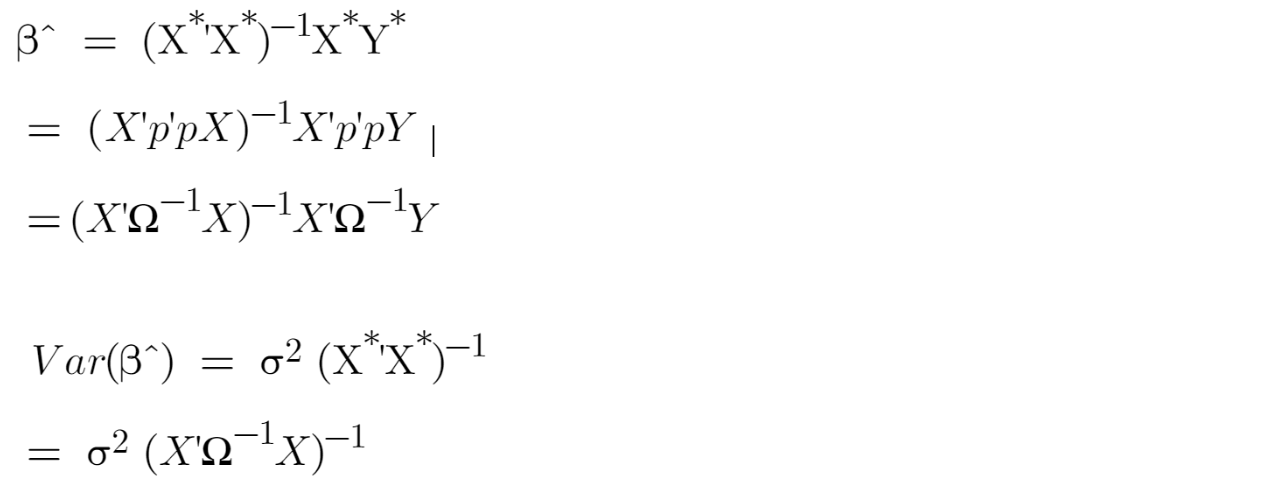
The transformed model satisfies the homoscedastic assumption, therefore, the OLS estimator for the transformed model (i.e., GLS estimator) is efficient. GLS estimator can be computed as

If we know the value of σ2Ω or Σ, we can just plug their values into a closed-form solution to find the GLS estimator.

If we don’t know the value of σ2Ω or Σ, the million-dollar question is “can we estimate their values?” The answer is YES. A common way to handle this kind of situation of using Feasible GLS (FGLS).

FGLS under Heteroskedasticity

As discussed in Wooldridge’s Introductory Econometrics: A Modern Approach, we can assume that

Let’s call the estimate of u², the weight, W, in the FGLS model (aka, Weighted Least Squares Estimation (WLS)).

A Feasible GLS Procedure to correct for Heteroskedasticity:

Step 1: Let run OLS as is and obtain the residuals, i.e., Ui hat.

Step 2: we create a new variable by first squaring the residuals and then taking the natural log.

Step 3: Regress this newly created variable on Xs, then predict their fitted values.

Step 4: Exponentiate the fitted value from step 3 and call it Weight, W. Then create a new matrix p, (i.e., N x N matrix)

Step 5: Transform both Y and X by multiplying the new matrix p.

Step 6: Apply OLS on the transformed model, β hat that we get would be an efficient GLS estimator.

FGLS under Autocorrelation

For most time-series data with autocorrelation, first-order autoregressive disturbances (i.e., AR(1)) correction would be sufficient. We have

Step 1: Let run OLS as is and obtain the residual vector e

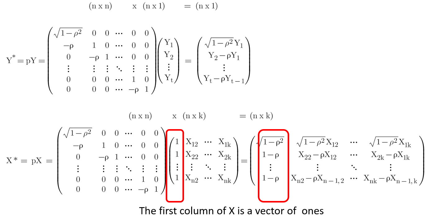
Step 2: estimate ρ by r, then create a new matrix p, (i.e., N x N matrix)

Step 3: Transform both Y and X by multiplying the new matrix p. The first observation is different from other observations. We can ignore the first observation (i.e., t=1) for our application.

Step 4: Apply OLS on the transformed model and obtain the GLS estimator.

When there is Heteroskedasticity in the linear regression model, the variance of error terms won’t be constant and when there is autocorrelation, the covariance of error terms are not zeros.

Under Heteroskedasticity or Autocorrelation, the OLS estimator would still be unbiased, but no longer efficient, meaning it won’t have the least variance.

To address the issues of Heteroskedasticity or Autocorrelation, we can either obtain robust standard error for the OLS estimator or to make the estimator more efficient, we can step up to obtain a GLS estimator by FGLS.

Here are some related posts you can explore if you’re interested in this topic.

You can sign up for a membership to unlock full access to my articles, and have unlimited access to everything on Medium. Please subscribe if you’d like to get an email notification whenever I post a new article.

Understand OLS Linear Regression with a bit of math

Heteroskedasticity and Autocorrelation are unavoidable issues we need to address when setting up a linear regression. In this article, let’s dive deeper into what are Heteroskedasticity and Autocorrelation, what are the Consequences, and remedies to handle issues.

A typical linear regression takes the form as follows. The response variable (i.e., Y) is explained as a linear combination of explanatory variables (e.g., the intercept, X1, X2, X3, …) and ε is the error term (i.e., a random variable) that represents the difference between the fitted response value and the actual response value.

Homoscedasticity

Under the assumption of Homoscedasticity, the error term should have constant variance and iid. In other words, the diagonal values in the variance-covariance matrix of the error term should be constant and off-diagonal values should be all 0.

Heteroskedasticity

In the real world, Homoscedasticity assumption may not be plausible. The variance of the error terms may not remain the same. Sometimes the variance of the error terms depends on the explanatory variable in the model.

For example, the number of bedrooms is usually used to predict house prices, we see that the prediction error is larger for houses with 6+ bedrooms than the ones with 2 bedrooms because houses with 6+ bedrooms are typically worth a lot more than 2-bedroom houses, therefore, have larger unexplained and sometimes irreducible price variance, which leaks into the error term.

We call the error term whose variances are NOT constant across observations Heteroskedastic error. This property is called Heteroskedasticity.

Autocorrelation

When there is autocorrelation in the model, the error terms are correlated. It means off-diagonal values of the covariance matrix of error terms are NOT all 0s.

There are some possible sources of autocorrelation. In the time-series data, time is the factor that produces autocorrelation. For example, the current stock price is influenced by the prices from previous trading days (e.g., the stock price is more likely to fall after a huge price hike). In the cross-section data, the neighboring units tend to have similar characteristics.

Remedy 1: Heteroskedasticity-consistent (HC) and Heteroskedasticity- Autocorrelation-consistent (HAC) Standard Errors

Under Heteroskedasticity or Autocorrelation, we can still use the inefficient OLS estimator, but many literatures suggest using Heteroskedasticity-consistent (HC) standard errors (aka, robust standard errors, White standard errors) or Heteroskedasticity- Autocorrelation-consistent (HAC) Standard Errors (aka, Newey-West Standard Error) that allow for the presence of Heteroskedasticity or Autocorrelation. These are the easiest and most common solutions.

Many econometricians argue that one should always use robust standard errors because one never can rely on Homoskedasticity.

Remedy 2: Generalized Least Square (GLS) and Feasible GLS (FGLS)

Instead of accepting an inefficient OLS estimator and correcting the standard errors, we can correct Heteroskedasticity or Autocorrelation by using a fully efficient estimator (i.e., unbiased and with the least variance) using Generalized Least Square (GLS).

Under Heteroskedasticity or Autocorrelation, although the OLS estimator and GLS estimator both are unbiased, the GLS estimator has a smaller variance than the OLS estimator.

If there is Heteroskedasticity or Autocorrelation and we either know the variance-covariance matrix of the error term or can estimate it empirically, then we can convert it into a homoscedastic model.

Q: Is the transformed model homoscedastic?

A: Yes, the error terms in the transformed model have constant variances and iid.

The transformed model satisfies the homoscedastic assumption, therefore, the OLS estimator for the transformed model (i.e., GLS estimator) is efficient. GLS estimator can be computed as

If we know the value of σ2Ω or Σ, we can just plug their values into a closed-form solution to find the GLS estimator.

If we don’t know the value of σ2Ω or Σ, the million-dollar question is “can we estimate their values?” The answer is YES. A common way to handle this kind of situation of using Feasible GLS (FGLS).

FGLS under Heteroskedasticity

As discussed in Wooldridge’s Introductory Econometrics: A Modern Approach, we can assume that

Let’s call the estimate of u², the weight, W, in the FGLS model (aka, Weighted Least Squares Estimation (WLS)).

A Feasible GLS Procedure to correct for Heteroskedasticity:

Step 1: Let run OLS as is and obtain the residuals, i.e., Ui hat.

Step 2: we create a new variable by first squaring the residuals and then taking the natural log.

Step 3: Regress this newly created variable on Xs, then predict their fitted values.

Step 4: Exponentiate the fitted value from step 3 and call it Weight, W. Then create a new matrix p, (i.e., N x N matrix)

Step 5: Transform both Y and X by multiplying the new matrix p.

Step 6: Apply OLS on the transformed model, β hat that we get would be an efficient GLS estimator.

FGLS under Autocorrelation

For most time-series data with autocorrelation, first-order autoregressive disturbances (i.e., AR(1)) correction would be sufficient. We have

Step 1: Let run OLS as is and obtain the residual vector e

Step 2: estimate ρ by r, then create a new matrix p, (i.e., N x N matrix)

Step 3: Transform both Y and X by multiplying the new matrix p. The first observation is different from other observations. We can ignore the first observation (i.e., t=1) for our application.

Step 4: Apply OLS on the transformed model and obtain the GLS estimator.

When there is Heteroskedasticity in the linear regression model, the variance of error terms won’t be constant and when there is autocorrelation, the covariance of error terms are not zeros.

Under Heteroskedasticity or Autocorrelation, the OLS estimator would still be unbiased, but no longer efficient, meaning it won’t have the least variance.

To address the issues of Heteroskedasticity or Autocorrelation, we can either obtain robust standard error for the OLS estimator or to make the estimator more efficient, we can step up to obtain a GLS estimator by FGLS.

Here are some related posts you can explore if you’re interested in this topic.

You can sign up for a membership to unlock full access to my articles, and have unlimited access to everything on Medium. Please subscribe if you’d like to get an email notification whenever I post a new article.