
Neural Network Representations – DZone
Trained neural networks arrive at solutions that achieve superhuman performance on an increasing number of tasks. It would be at least interesting and probably important to understand these solutions.
Interesting, in the spirit of curiosity and getting answers to questions like, “Are there human-understandable algorithms that capture how object-detection nets work?”[a] This would add a new modality of use to our relationship with neural nets from just querying for answers (Oracle Models) or sending on tasks (Agent Models) to acquiring an enriched understanding of our world by studying the interpretable internals of these networks’ solutions (Microscope Models). [1]
And important in its use in the pursuit of the kinds of standards that we (should?) demand of increasingly powerful systems, such as operational transparency, and guarantees on behavioral bounds. A common example of an idealized capability we could hope for is “lie detection” by monitoring the model’s internal state. [2]
Mechanistic interpretability (mech interp) is a subfield of interpretability research that seeks a granular understanding of these networks.
One could describe two categories of mech interp inquiry:
- Representation interpretability: Understanding what a model sees and how it does; i.e., what information have models found important to look for in their inputs and how is this information represented internally?
- Algorithmic interpretability: Understanding how this information is used for computation across the model to result in some observed outcome
Figure 1: “A Conscious Blackbox,” the cover graphic for James C. Scott’s Seeing Like a State (1998)
This post is concerned with representation interpretability. Structured as an exposition of neural network representation research [b], it discusses various qualities of model representations which range in epistemic confidence from the obvious to the speculative and the merely desired.
Notes:
- I’ll use “Models/Neural Nets” and “Model Components” interchangeably. A model component can be thought of as a layer or some other conceptually meaningful ensemble of layers in a network.
- Until properly introduced with a technical definition, I use expressions like “input-properties” and “input-qualities” in place of the more colloquially used “feature.”
Now, to some foundational hypotheses about neural network representations.
Decomposability
The representations of inputs to a model are a composition of encodings of discrete information. That is, when a model looks for different qualities in an input, the representation of the input in some component of the model can be described as a combination of its representations of these qualities. This makes (de)composability a corollary of “encoding discrete information”- the model’s ability to represent a fixed set of different qualities as seen in its inputs.
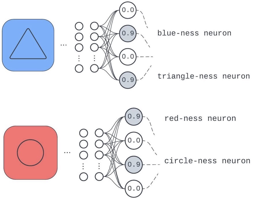
Figure 2: A model layer trained on a task that needs it to care about background colors (trained on only blue and red) and center shapes (only circles and triangles)
The component has dedicated a different neuron to the input qualities: “background color is composed of red,” “background color is composed of blue,” “center object is a circle,” and “center object is a triangle.”
Consider the alternative: if a model didn’t identify any predictive discrete qualities of inputs in the course of training. To do well on a task, the network would have to work like a lookup table with its keys as the bare input pixels (since it can’t glean any discrete properties more interesting than “the ordered set of input pixels”) pointing to unique identifiers. We have a name for this in practice: memorizing. Therefore, saying, “Model components learn to identify useful discrete qualities of inputs and compose them to get internal representations used for downstream computation,” is not far off from saying “Sometimes, neural nets don’t completely memorize.”
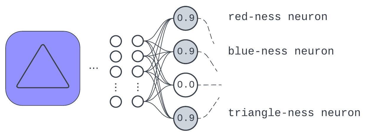
Figure 3: An example of how learning discrete input qualities affords generalization or robustness
This example test input, not seen in training, has a representation expressed in the learned qualities. While the model might not fully appreciate what “purple” is, it’ll be better off than if it was just trying to do a table lookup for input pixels.
Revisiting the hypothesis:
“The representations of inputs to a model are a composition of encodings of discrete information.”
While, as we’ve seen, this verges on the obvious; it provides a template for introducing stricter specifications deserving of study.
The first of these specification revisits looks at “…are a composition of encodings…” What is observed, speculated, and hoped for about the nature of these compositions of the encodings?
Linearity
To recap decomposition, we expect (non-memorizing) neural networks to identify and encode varied information from input qualities/properties. This implies that any activation state is a composition of these encodings.
Figure 4: What the decomposability hypothesis suggests
What is the nature of this composition? In this context, saying a representation is linear suggests the information of discrete input qualities are encoded as directions in activation space and they are composed into a representation by a vector sum:
We’ll investigate both claims.
Claim #1: Encoded Qualities Are Directions in Activation Space
Composability already suggests that the representation of input in some model components (a vector in activation space) is composed of discrete encodings of input qualities (other vectors in activation space). The additional thing said here is that in a given input-quality encoding, we can think of there being some core essence of the quality which is the vector’s direction. This makes any particular encoding vector just a scaled version of this direction (unit vector.)
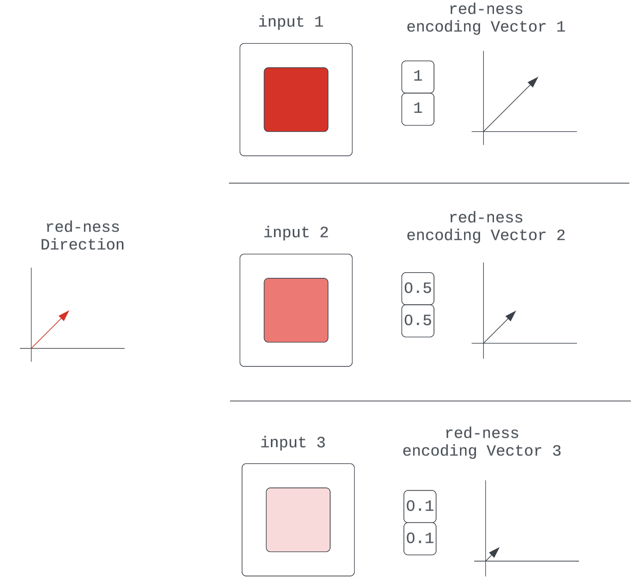
Figure 5: Various encoding vectors for the red-ness quality in the input
They are all just scaled representations of some fundamental red-ness unit vector, which specifies direction.
This is simply a generalization of the composability argument that says neural networks can learn to make their encodings of input qualities “intensity”-sensitive by scaling some characteristic unit vector.
Alternative Impractical Encoding Regimes
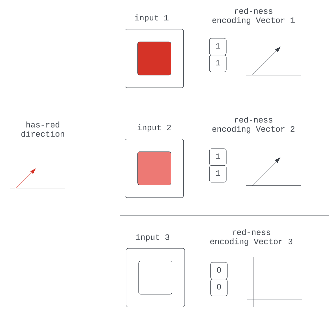
Figure 6a
An alternative encoding scheme could be that all we can get from models are binary encodings of properties; e.g., “The Red values in this RGB input are Non-zero.” This is clearly not very robust.
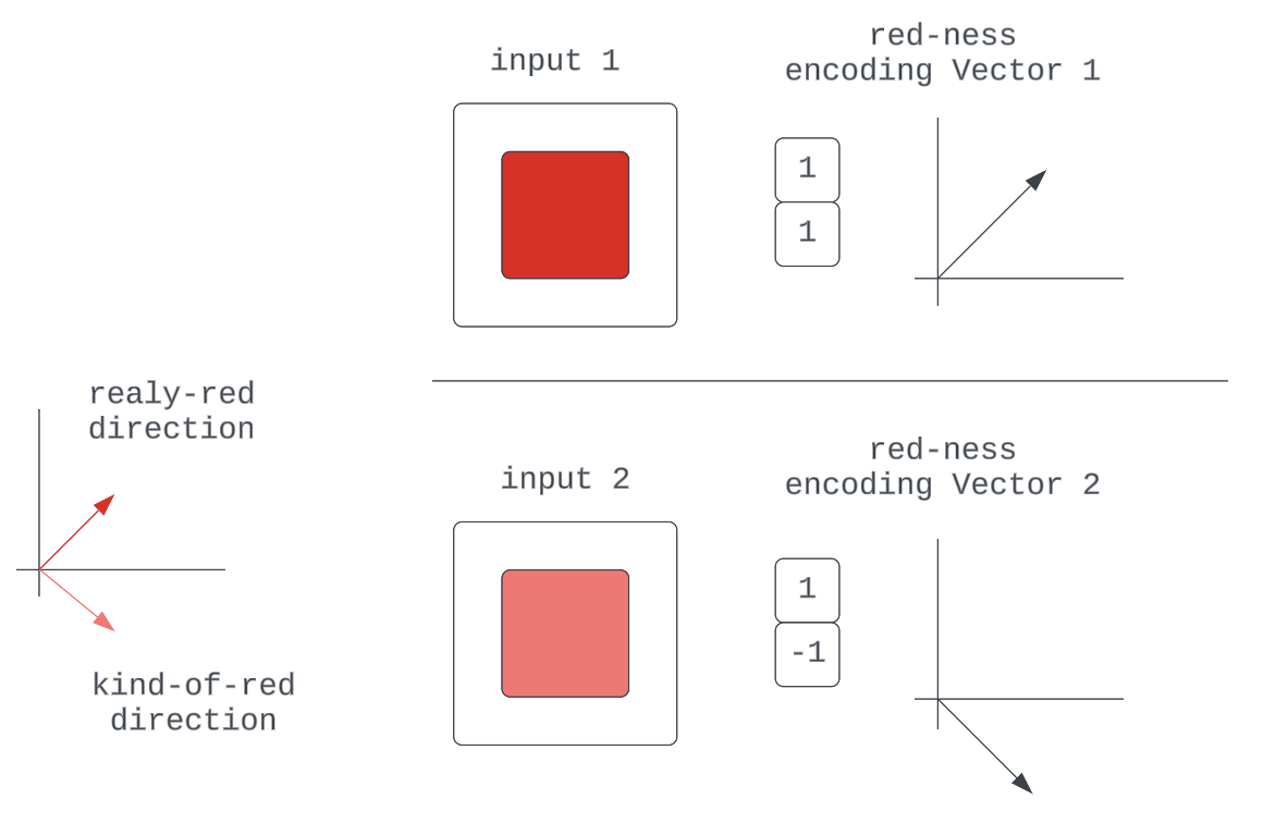
Figure 6b
Another is that we have multiple unique directions for qualities that could be described by mere differences in scale of some more fundamental quality: “One Neuron for “kind-of-red” for 0-127 in the RGB input, another for “really-red” for 128-255 in the RGB input.” We’d run out of directions fairly quickly.
Claim #2: These Encodings Are Composed as a Vector Sum
Now, this is the stronger of the two claims as it is not necessarily a consequence of anything introduced thus far.
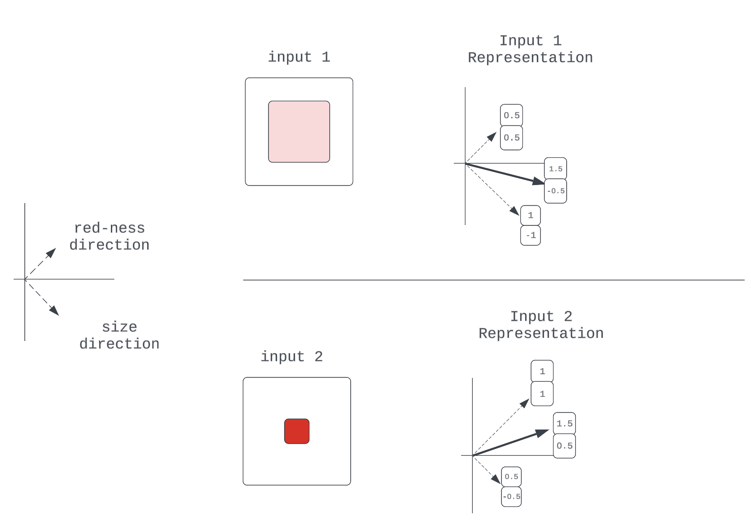
Figure 7: An example of 2-property representation
Note: We assume independence between properties, ignoring the degenerate case where a size of zero implies the color is not red (nothing).
A vector sum might seem like the natural (if not only) thing a network could do to combine these encoding vectors. To appreciate why this claim is worth verifying, it’ll be worth investigating if alternative non-linear functions could also get the job done. Recall that the thing we want is a function that combines these encodings at some component in the model in a way that preserves information for downstream computation. So this is effectively an information compression problem.
As discussed in Elhage et al [3a], the following non-linear compression scheme could get the job done:
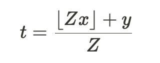
Where we seek to compress values x and y into t. The value of Z is chosen according to the required floating-point precision needed for compressions.
# A Python Implementation

from math import floor

def compress_values(x1, x2, precision=1):
    z = 10 ** precision
    compressed_val = (floor(z * x1) + x2) / z
    return round(compressed_val, precision * 2)

def recover_values(compressed_val, precision=1):
    z = 10 ** precision
    x2_recovered = (compressed_val * z) - floor(compressed_val * z)
    x1_recovered = compressed_val - (x2_recovered / z)
    return round(x1_recovered, precision), round(x2_recovered, precision)

# Now to compress vectors a and b

a = [0.3, 0.6]
b = [0.2, 0.8]

compressed_a_b = [compress_values(a[0], b[0]), compress_values(a[1], b[1])]
# Returned [0.32, 0.68]

recovered_a, recovered_b = (
    [x, y] for x, y in zip(
        recover_values(compressed_a_b[0]),
        recover_values(compressed_a_b[1])
    )
)
# Returned ([0.3, 0.6], [0.2, 0.8])

assert all([recovered_a == a, recovered_b == b])
As demonstrated, we’re able to compress and recover vectors a and b just fine, so this is also a viable way of compressing information for later computation using non-linearities like the floor() function that neural networks can approximate. While this seems a little more tedious than just adding vectors, it shows the network does have options. This calls for some evidence and further arguments in support of linearity.
Evidence of Linearity
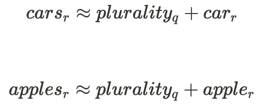
The often-cited example of a model component exhibiting strong linearity is the embedding layer in language models [4], where relationships like the following exist between representations of words:
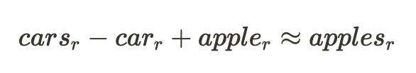
This example would hint at the following relationship between the quality of $plurality$ in the input words and the rest of their representation:
Okay, so that’s some evidence for one component in a type of neural network having linear representations. The broad outline of arguments for this being prevalent across networks is that linear representations are both the more natural and performant [3b][3a] option for neural networks to settle on.
How Important for Interpretability Is It That This Is True?
If non-linear compression is prevalent across networks, there are two alternative regimes in which networks could operate:
- Computation is still mostly done on linear variables: In this regime, while the information is encoded and moved between components non-linearly, the model components would still decompress the representations to run linear computations. From an interpretability standpoint, while this needs some additional work to reverse engineer the decompression operation, this wouldn’t pose too high a barrier.
![Non-linear compression and propagation intervened by linear computation]() Figure 8:Non-linear compression and propagation intervened by linear computation
Figure 8:Non-linear compression and propagation intervened by linear computation - Computation is done in a non-linear state: The model figures out a way to do computations directly on the non-linear representation. This would pose a challenge needing new interpretability methods. However, based on arguments discussed earlier about model architecture affordances this is expected to be unlikely.
![]()
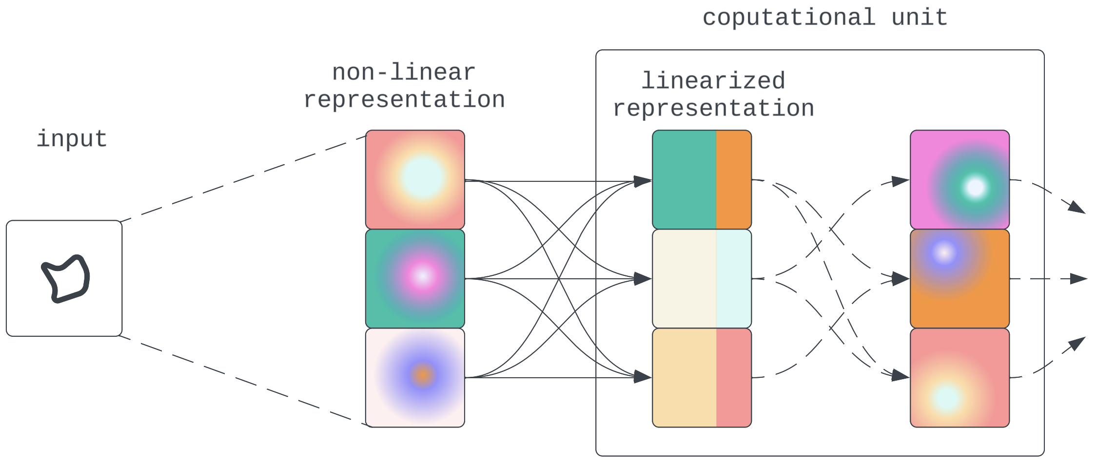 Figure 8:Non-linear compression and propagation intervened by linear computation
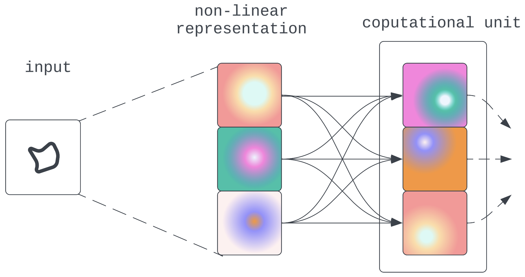
Figure 9: Direct non-linear computation
Features
As promised in the introduction, after avoiding the word “feature” this far into the post, we’ll introduce it properly. As a quick aside, I think the engagement of the research community on the topic of defining what we mean when we use the word “feature” is one of the things that makes mech interp, as a pre-paradigmatic science, exciting. While different definitions have been proposed [3c] and the final verdict is by no means out, in this post and others to come on mech interp, I’ll be using the following:
“The features of a given neural network constitute a set of all the input qualities the network would dedicate a neuron to if it could.”
We’ve already discussed the idea of networks necessarily encoding discrete qualities of inputs, so the most interesting part of the definition is, “…would dedicate a neuron to if it could.”
What Is Meant by “…Dedicate a Neuron To…”?
In a case where all quality-encoding directions are unique one-hot vectors in activation space ([0, 1] and [1, 0], for example) the neurons are said to be basis-aligned; i.e., one neuron’s activation in the network independently represents the intensity of one input quality.
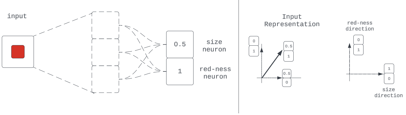
Figure 10: Example of a representation with basis-aligned neurons
Note that while sufficient, this property is not necessary for lossless compression of encodings with vector addition. The core requirement is that these feature directions be orthogonal. The reason for this is the same as when we explored the non-linear compression method: we want to completely recover each encoded feature downstream.
Basis Vectors
Following the Linearity hypothesis, we expect the activation vector to be a sum of all the scaled feature directions:
Given an activation vector (which is what we can directly observe when our network fires), if we want to know the activation intensity of some feature in the input, all we need is the feature’s unit vector, feature^j_d: (where the character “.” in the following expression is the vector dot product.)
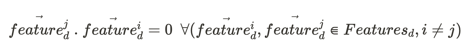
If all the feature unit vectors of that network component (making up the set, Features_d) are orthogonal to each other:
And, for any vector:
These simplify our equation to give an expression for our feature intensity feature^j_i:
Allowing us to fully recover our compressed feature:
All that was to establish the ideal property of orthogonality between feature directions. This means even though the idea of “one neuron firing by x-much == one feature is present by x-much” is pretty convenient to think about, there are other equally performant feature directions that don’t have their neuron-firing patterns aligning this cleanly with feature patterns. (As an aside, it turns out basis-aligned neurons don’t happen that often. [3d])
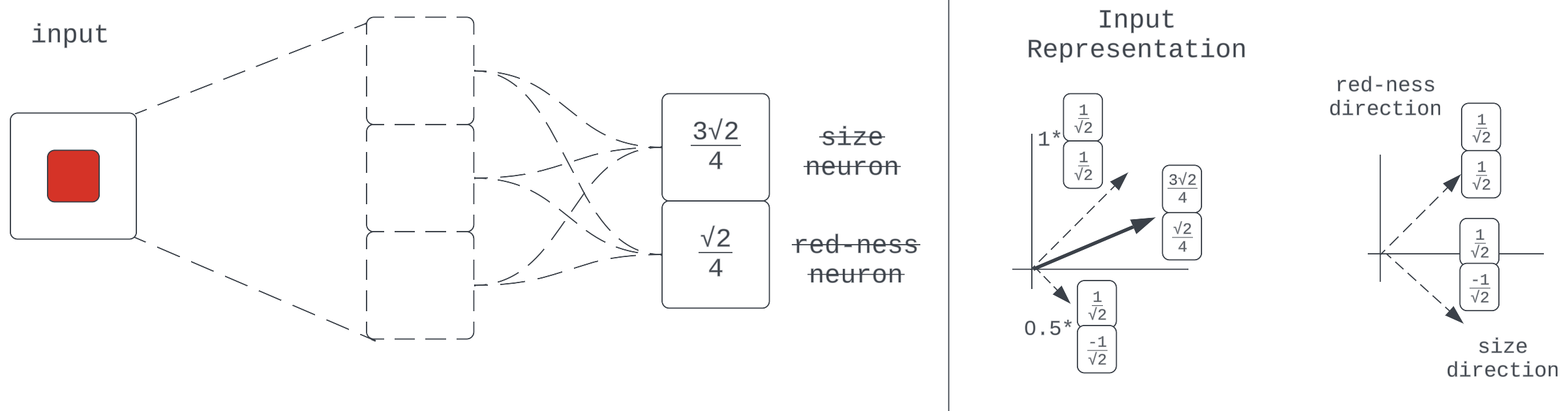
Fig 11: Orthogonal feature directions from non-basis-aligned neurons
With this context, the request: ”dedicate a neuron to…” might seem arbitrarily specific. Perhaps “dedicate an extra orthogonal direction vector” would be sufficient to accommodate an additional quality. But as you probably already know, orthogonal vectors in a space don’t grow on trees. A 2-dimensional space can only have 2 orthogonal vectors at a time, for example. So to make more room, we might need an extra dimension, i.e [X X] -> [X X X] which is tantamount to having an extra neuron dedicated to this feature.
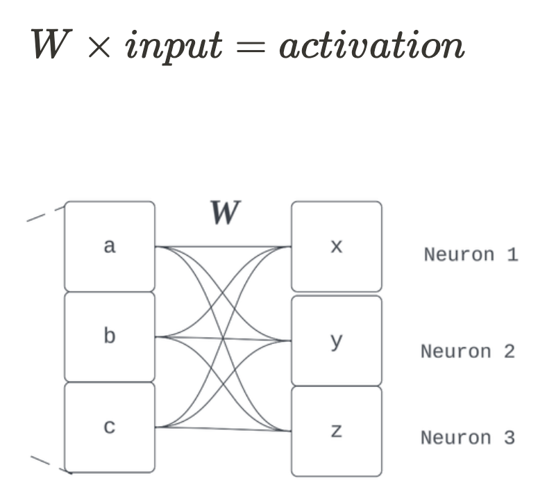
How Are These Features Stored in Neural Networks?
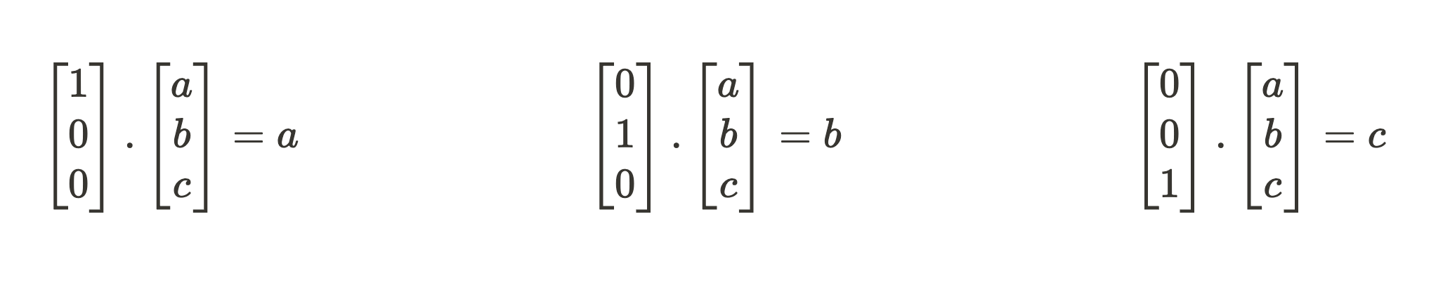
To touch grass quickly, what does it mean when a model component has learned 3 orthogonal feature directions {[1 0 0], [0 1 0], [0 0 1]} for compressing an input vector [a b c]?
To get the compressed activation vector, we expect a series of dot products with each feature direction to get our feature scale.
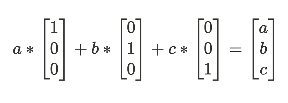
Now we just have to sum up our scaled-up feature directions to get our “compressed” activation state. In this toy example, the features are just the vector values so lossless decompressing gets us what we started with.
The question is: what does this look like in a model? The above sequence of transformations of dot products followed by a sum is equivalent to the operations of the deep learning workhorse: matrix multiplication.
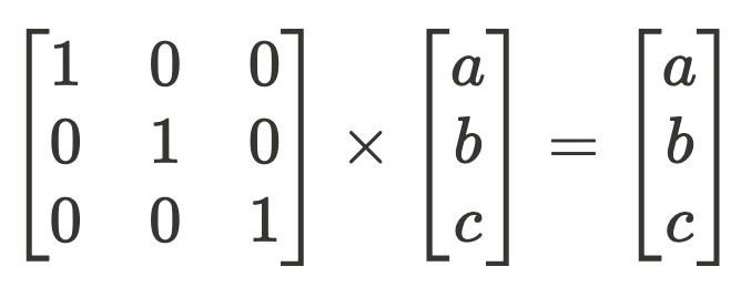
The earlier sentence, “…a model component has learned 3 orthogonal feature directions,” should have been a giveaway. Models store their learnings in weights, and so our feature vectors are just the rows of this layer’s learned weight matrix, W.
Why didn’t I just say the whole time, “Matrix multiplication. End of section.” Because we don’t always have toy problems in the real world. The learned features aren’t always stored in just one set of weights. It could (and usually does) involve an arbitrarily long sequence of linear and non-linear compositions to arrive at some feature direction (but the key insight of decompositional linearity is that this computation can be summarised by a direction used to compose some activation). The promise of linearity we discussed only has to do with how feature representations are composed. For example, some arbitrary vector is more likely to not be hanging around for discovery by just reading one row of a layer’s weight matrix, but the computation to encode that feature is spread across several weights and model components. So we had to address features as arbitrary strange directions in activation space because they often are. This point brings the proposed dichotomy between representation and algorithmic interpretability into question.
Back to our working definition of features:
“The features of a given neural network constitute a set of all the input qualities the network would dedicate a neuron to if it could.”
On the Conditional Clause: “…Would Dedicate a Neuron to if It Could…”
You can think of this definition of a feature as a bit of a set-up for an introduction to a hypothesis that addresses its counterfactual: What happens when a neural network cannot provide all its input qualities with dedicated neurons?
Superposition
Thus far, our model has done fine on the task that required it to compress and propagate 2 learned features — “size” and “red-ness” — through a 2-dimensional layer. What happens when a new task requires the compression and propagation of an additional feature like the x-displacement of the center of the square?
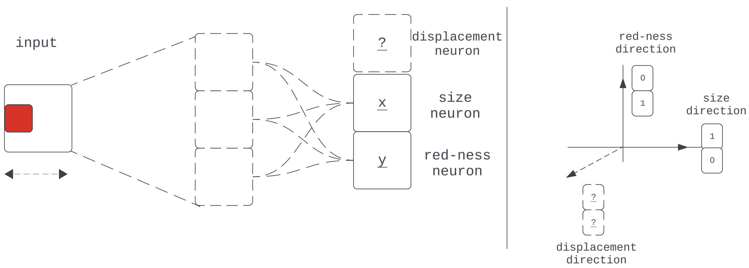
Figure 12
This shows our network with a new task, requiring it to propagate one more learned property of the input: center x-displacement. We’ve returned to using neuron-aligned bases for convenience.
Before we go further with this toy model, it would be worth thinking through if there are analogs of this in large real-world models. Let’s take the large language model GPT2 small [5]. Do you think, if you had all week, you could think of up to 769 useful features of an arbitrary 700-word query that would help predict the next token (e.g., “is a formal letter,” “contains how many verbs,” “is about about ‘Chinua Achebe,’” etc.)? Even if we ignored the fact that feature discovery was one of the known superpowers of neural networks [c] and assumed GPT2-small would also end up with only 769 useful input features to encode, we’d have a situation much like our toy problem above. This is because GPT2 has —at the narrowest point in its architecture— only 768 neurons to work with, just like our toy problem has 2 neurons but needs to encode information about 3 features. [d]
So this whole “model component encodes more features it has neurons” business should be worth looking into. It probably also needs a shorter name. That name is the Superposition hypothesis. Considering the above thought experiment with GPT2 Small, it would seem this hypothesis is just stating the obvious- that models are somehow able to represent more input qualities (features) than they have dimensions for.
What Exactly Is Hypothetical About Superposition?
There’s a reason I introduced it this late in the post: it depends on other abstractions that aren’t necessarily self-evident. The most important is the prior formulation of features. It assumes linear decomposition- the expression of neural net representations as sums of scaled directions representing discrete qualities of their inputs. These definitions might seem circular, but they’re not if defined sequentially:
If you conceive of neural networks as encoding discrete information of inputs called Features as directions in activation space, then when we suspect the model has more of these features than it has neurons, we call this Superposition.
A Way Forward
As we’ve seen, it would be convenient if the features of a model were aligned with neurons and necessary for them to be orthogonal vectors to allow lossless recovery from compressed representations. So to suggest this isn’t happening poses difficulties to interpretation and raises questions on how networks can pull this off anyway.
Further development of the hypothesis provides a model for thinking about why and how superposition happens, clearly exposes the phenomenon in toy problems, and develops promising methods for working around barriers to interpretability [6]. More on this in a future post.
Footnotes
[a] That is, algorithms more descriptive than “Take this Neural Net architecture and fill in its weights with these values, then do a forward pass.”
[b] Primarily from ideas introduced in Toy Models of Superposition
[c] This refers specifically to the codification of features as their superpower. Humans are pretty good at predicting the next token in human text; we’re just not good at writing programs for extracting and representing this information vector space. All of that is hidden away in the mechanics of our cognition.
[d] Technically, the number to compare the 768-dimension residual stream width to is the maximum number of features we think *any* single layer would have to deal with at a time. If we assume equal computational workload between layers and assume each batch of features was built based on computations on the previous, for the 12-layer GPT2 model, this would be 12 * 768 = 9,216 features you’d need to think up.
References
[1] Chris Olah on Mech Interp – 80000 Hours
[3] Toy Models of Superposition
[3c] What are Features?
[3d] Definitions and Motivation
[4] Linguistic regularities in continuous space word representations: Mikolov, T., Yih, W. and Zweig, G., 2013. Proceedings of the 2013 conference of the North American chapter of the Association for Computational Linguistics: Human language technologies, pp. 746–751.
[5] Language Models are Unsupervised Multitask Learners: Alec Radford, Jeffrey Wu, Rewon Child, David Luan, Dario Amodei, Ilya Sutskever
[6] Towards Monosemanticity: Decomposing Language Models With Dictionary Learning
Trained neural networks arrive at solutions that achieve superhuman performance on an increasing number of tasks. It would be at least interesting and probably important to understand these solutions.
Interesting, in the spirit of curiosity and getting answers to questions like, “Are there human-understandable algorithms that capture how object-detection nets work?”[a] This would add a new modality of use to our relationship with neural nets from just querying for answers (Oracle Models) or sending on tasks (Agent Models) to acquiring an enriched understanding of our world by studying the interpretable internals of these networks’ solutions (Microscope Models). [1]
And important in its use in the pursuit of the kinds of standards that we (should?) demand of increasingly powerful systems, such as operational transparency, and guarantees on behavioral bounds. A common example of an idealized capability we could hope for is “lie detection” by monitoring the model’s internal state. [2]
Mechanistic interpretability (mech interp) is a subfield of interpretability research that seeks a granular understanding of these networks.
One could describe two categories of mech interp inquiry:
- Representation interpretability: Understanding what a model sees and how it does; i.e., what information have models found important to look for in their inputs and how is this information represented internally?
- Algorithmic interpretability: Understanding how this information is used for computation across the model to result in some observed outcome
Figure 1: “A Conscious Blackbox,” the cover graphic for James C. Scott’s Seeing Like a State (1998)
This post is concerned with representation interpretability. Structured as an exposition of neural network representation research [b], it discusses various qualities of model representations which range in epistemic confidence from the obvious to the speculative and the merely desired.
Notes:
- I’ll use “Models/Neural Nets” and “Model Components” interchangeably. A model component can be thought of as a layer or some other conceptually meaningful ensemble of layers in a network.
- Until properly introduced with a technical definition, I use expressions like “input-properties” and “input-qualities” in place of the more colloquially used “feature.”
Now, to some foundational hypotheses about neural network representations.
Decomposability
The representations of inputs to a model are a composition of encodings of discrete information. That is, when a model looks for different qualities in an input, the representation of the input in some component of the model can be described as a combination of its representations of these qualities. This makes (de)composability a corollary of “encoding discrete information”- the model’s ability to represent a fixed set of different qualities as seen in its inputs.
Figure 2: A model layer trained on a task that needs it to care about background colors (trained on only blue and red) and center shapes (only circles and triangles)
The component has dedicated a different neuron to the input qualities: “background color is composed of red,” “background color is composed of blue,” “center object is a circle,” and “center object is a triangle.”
Consider the alternative: if a model didn’t identify any predictive discrete qualities of inputs in the course of training. To do well on a task, the network would have to work like a lookup table with its keys as the bare input pixels (since it can’t glean any discrete properties more interesting than “the ordered set of input pixels”) pointing to unique identifiers. We have a name for this in practice: memorizing. Therefore, saying, “Model components learn to identify useful discrete qualities of inputs and compose them to get internal representations used for downstream computation,” is not far off from saying “Sometimes, neural nets don’t completely memorize.”
Figure 3: An example of how learning discrete input qualities affords generalization or robustness
This example test input, not seen in training, has a representation expressed in the learned qualities. While the model might not fully appreciate what “purple” is, it’ll be better off than if it was just trying to do a table lookup for input pixels.
Revisiting the hypothesis:
“The representations of inputs to a model are a composition of encodings of discrete information.”
While, as we’ve seen, this verges on the obvious; it provides a template for introducing stricter specifications deserving of study.
The first of these specification revisits looks at “…are a composition of encodings…” What is observed, speculated, and hoped for about the nature of these compositions of the encodings?
Linearity
To recap decomposition, we expect (non-memorizing) neural networks to identify and encode varied information from input qualities/properties. This implies that any activation state is a composition of these encodings.
Figure 4: What the decomposability hypothesis suggests
What is the nature of this composition? In this context, saying a representation is linear suggests the information of discrete input qualities are encoded as directions in activation space and they are composed into a representation by a vector sum:
We’ll investigate both claims.
Claim #1: Encoded Qualities Are Directions in Activation Space
Composability already suggests that the representation of input in some model components (a vector in activation space) is composed of discrete encodings of input qualities (other vectors in activation space). The additional thing said here is that in a given input-quality encoding, we can think of there being some core essence of the quality which is the vector’s direction. This makes any particular encoding vector just a scaled version of this direction (unit vector.)
Figure 5: Various encoding vectors for the red-ness quality in the input
They are all just scaled representations of some fundamental red-ness unit vector, which specifies direction.
This is simply a generalization of the composability argument that says neural networks can learn to make their encodings of input qualities “intensity”-sensitive by scaling some characteristic unit vector.
Alternative Impractical Encoding Regimes
Figure 6a
An alternative encoding scheme could be that all we can get from models are binary encodings of properties; e.g., “The Red values in this RGB input are Non-zero.” This is clearly not very robust.
Figure 6b
Another is that we have multiple unique directions for qualities that could be described by mere differences in scale of some more fundamental quality: “One Neuron for “kind-of-red” for 0-127 in the RGB input, another for “really-red” for 128-255 in the RGB input.” We’d run out of directions fairly quickly.
Claim #2: These Encodings Are Composed as a Vector Sum
Now, this is the stronger of the two claims as it is not necessarily a consequence of anything introduced thus far.
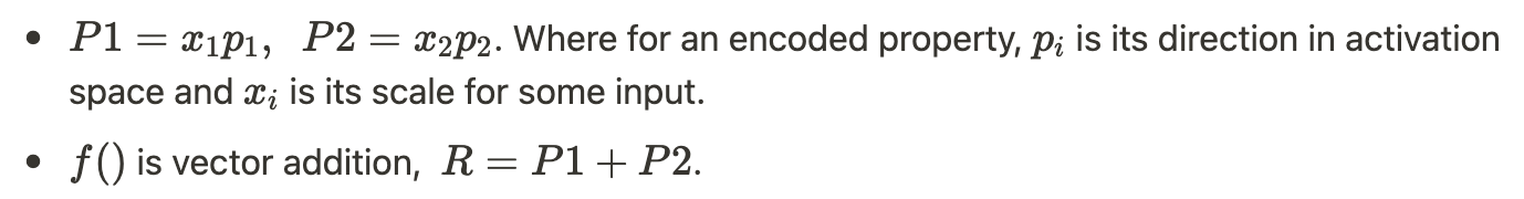
Figure 7: An example of 2-property representation
Note: We assume independence between properties, ignoring the degenerate case where a size of zero implies the color is not red (nothing).
A vector sum might seem like the natural (if not only) thing a network could do to combine these encoding vectors. To appreciate why this claim is worth verifying, it’ll be worth investigating if alternative non-linear functions could also get the job done. Recall that the thing we want is a function that combines these encodings at some component in the model in a way that preserves information for downstream computation. So this is effectively an information compression problem.
As discussed in Elhage et al [3a], the following non-linear compression scheme could get the job done:
Where we seek to compress values x and y into t. The value of Z is chosen according to the required floating-point precision needed for compressions.
# A Python Implementation

from math import floor

def compress_values(x1, x2, precision=1):
    z = 10 ** precision
    compressed_val = (floor(z * x1) + x2) / z
    return round(compressed_val, precision * 2)

def recover_values(compressed_val, precision=1):
    z = 10 ** precision
    x2_recovered = (compressed_val * z) - floor(compressed_val * z)
    x1_recovered = compressed_val - (x2_recovered / z)
    return round(x1_recovered, precision), round(x2_recovered, precision)

# Now to compress vectors a and b

a = [0.3, 0.6]
b = [0.2, 0.8]

compressed_a_b = [compress_values(a[0], b[0]), compress_values(a[1], b[1])]
# Returned [0.32, 0.68]

recovered_a, recovered_b = (
    [x, y] for x, y in zip(
        recover_values(compressed_a_b[0]),
        recover_values(compressed_a_b[1])
    )
)
# Returned ([0.3, 0.6], [0.2, 0.8])

assert all([recovered_a == a, recovered_b == b])
As demonstrated, we’re able to compress and recover vectors a and b just fine, so this is also a viable way of compressing information for later computation using non-linearities like the floor() function that neural networks can approximate. While this seems a little more tedious than just adding vectors, it shows the network does have options. This calls for some evidence and further arguments in support of linearity.
Evidence of Linearity
The often-cited example of a model component exhibiting strong linearity is the embedding layer in language models [4], where relationships like the following exist between representations of words:
This example would hint at the following relationship between the quality of $plurality$ in the input words and the rest of their representation:
Okay, so that’s some evidence for one component in a type of neural network having linear representations. The broad outline of arguments for this being prevalent across networks is that linear representations are both the more natural and performant [3b][3a] option for neural networks to settle on.
How Important for Interpretability Is It That This Is True?
If non-linear compression is prevalent across networks, there are two alternative regimes in which networks could operate:
- Computation is still mostly done on linear variables: In this regime, while the information is encoded and moved between components non-linearly, the model components would still decompress the representations to run linear computations. From an interpretability standpoint, while this needs some additional work to reverse engineer the decompression operation, this wouldn’t pose too high a barrier.
![Non-linear compression and propagation intervened by linear computation]() Figure 8:Non-linear compression and propagation intervened by linear computation
Figure 8:Non-linear compression and propagation intervened by linear computation - Computation is done in a non-linear state: The model figures out a way to do computations directly on the non-linear representation. This would pose a challenge needing new interpretability methods. However, based on arguments discussed earlier about model architecture affordances this is expected to be unlikely.
![]()
Figure 9: Direct non-linear computation
Features
As promised in the introduction, after avoiding the word “feature” this far into the post, we’ll introduce it properly. As a quick aside, I think the engagement of the research community on the topic of defining what we mean when we use the word “feature” is one of the things that makes mech interp, as a pre-paradigmatic science, exciting. While different definitions have been proposed [3c] and the final verdict is by no means out, in this post and others to come on mech interp, I’ll be using the following:
“The features of a given neural network constitute a set of all the input qualities the network would dedicate a neuron to if it could.”
We’ve already discussed the idea of networks necessarily encoding discrete qualities of inputs, so the most interesting part of the definition is, “…would dedicate a neuron to if it could.”
What Is Meant by “…Dedicate a Neuron To…”?
In a case where all quality-encoding directions are unique one-hot vectors in activation space ([0, 1] and [1, 0], for example) the neurons are said to be basis-aligned; i.e., one neuron’s activation in the network independently represents the intensity of one input quality.
Figure 10: Example of a representation with basis-aligned neurons
Note that while sufficient, this property is not necessary for lossless compression of encodings with vector addition. The core requirement is that these feature directions be orthogonal. The reason for this is the same as when we explored the non-linear compression method: we want to completely recover each encoded feature downstream.
Basis Vectors
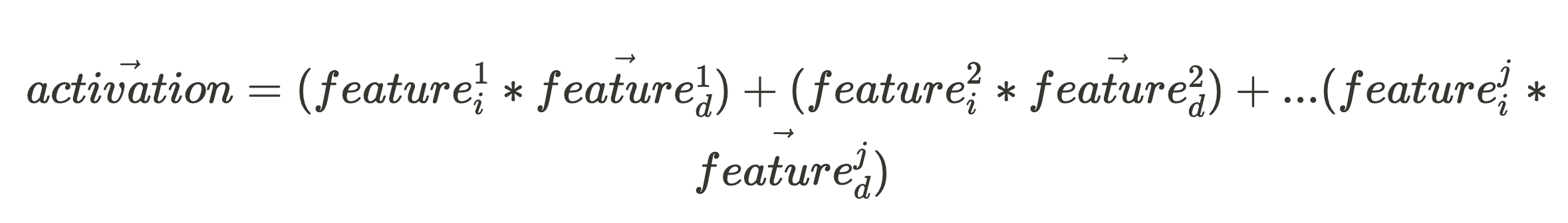
Following the Linearity hypothesis, we expect the activation vector to be a sum of all the scaled feature directions:
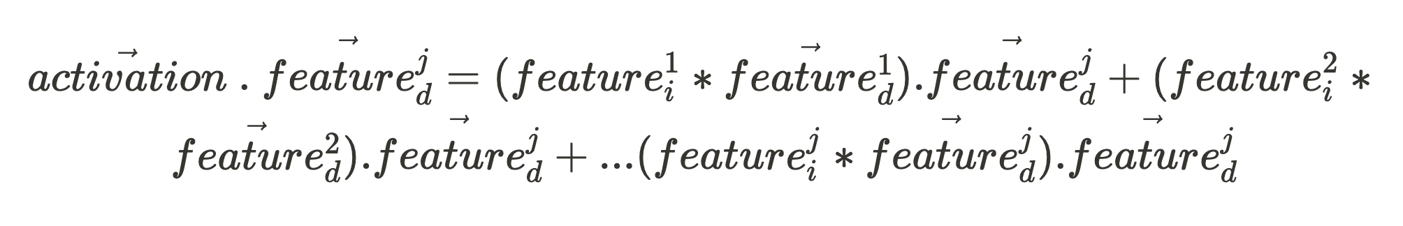
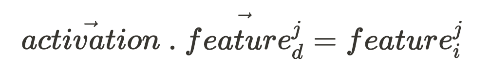
Given an activation vector (which is what we can directly observe when our network fires), if we want to know the activation intensity of some feature in the input, all we need is the feature’s unit vector, feature^j_d: (where the character “.” in the following expression is the vector dot product.)
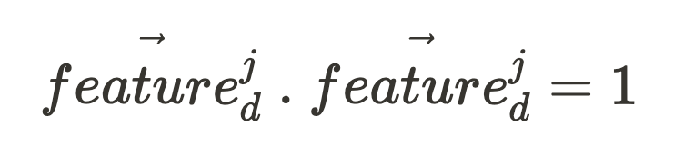
If all the feature unit vectors of that network component (making up the set, Features_d) are orthogonal to each other:
And, for any vector:
These simplify our equation to give an expression for our feature intensity feature^j_i:
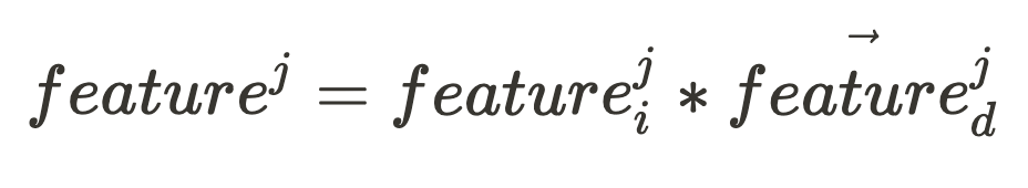
Allowing us to fully recover our compressed feature:
All that was to establish the ideal property of orthogonality between feature directions. This means even though the idea of “one neuron firing by x-much == one feature is present by x-much” is pretty convenient to think about, there are other equally performant feature directions that don’t have their neuron-firing patterns aligning this cleanly with feature patterns. (As an aside, it turns out basis-aligned neurons don’t happen that often. [3d])
Fig 11: Orthogonal feature directions from non-basis-aligned neurons
With this context, the request: ”dedicate a neuron to…” might seem arbitrarily specific. Perhaps “dedicate an extra orthogonal direction vector” would be sufficient to accommodate an additional quality. But as you probably already know, orthogonal vectors in a space don’t grow on trees. A 2-dimensional space can only have 2 orthogonal vectors at a time, for example. So to make more room, we might need an extra dimension, i.e [X X] -> [X X X] which is tantamount to having an extra neuron dedicated to this feature.
How Are These Features Stored in Neural Networks?
To touch grass quickly, what does it mean when a model component has learned 3 orthogonal feature directions {[1 0 0], [0 1 0], [0 0 1]} for compressing an input vector [a b c]?
To get the compressed activation vector, we expect a series of dot products with each feature direction to get our feature scale.
Now we just have to sum up our scaled-up feature directions to get our “compressed” activation state. In this toy example, the features are just the vector values so lossless decompressing gets us what we started with.
The question is: what does this look like in a model? The above sequence of transformations of dot products followed by a sum is equivalent to the operations of the deep learning workhorse: matrix multiplication.
The earlier sentence, “…a model component has learned 3 orthogonal feature directions,” should have been a giveaway. Models store their learnings in weights, and so our feature vectors are just the rows of this layer’s learned weight matrix, W.
Why didn’t I just say the whole time, “Matrix multiplication. End of section.” Because we don’t always have toy problems in the real world. The learned features aren’t always stored in just one set of weights. It could (and usually does) involve an arbitrarily long sequence of linear and non-linear compositions to arrive at some feature direction (but the key insight of decompositional linearity is that this computation can be summarised by a direction used to compose some activation). The promise of linearity we discussed only has to do with how feature representations are composed. For example, some arbitrary vector is more likely to not be hanging around for discovery by just reading one row of a layer’s weight matrix, but the computation to encode that feature is spread across several weights and model components. So we had to address features as arbitrary strange directions in activation space because they often are. This point brings the proposed dichotomy between representation and algorithmic interpretability into question.
Back to our working definition of features:
“The features of a given neural network constitute a set of all the input qualities the network would dedicate a neuron to if it could.”
On the Conditional Clause: “…Would Dedicate a Neuron to if It Could…”
You can think of this definition of a feature as a bit of a set-up for an introduction to a hypothesis that addresses its counterfactual: What happens when a neural network cannot provide all its input qualities with dedicated neurons?
Superposition
Thus far, our model has done fine on the task that required it to compress and propagate 2 learned features — “size” and “red-ness” — through a 2-dimensional layer. What happens when a new task requires the compression and propagation of an additional feature like the x-displacement of the center of the square?
Figure 12
This shows our network with a new task, requiring it to propagate one more learned property of the input: center x-displacement. We’ve returned to using neuron-aligned bases for convenience.
Before we go further with this toy model, it would be worth thinking through if there are analogs of this in large real-world models. Let’s take the large language model GPT2 small [5]. Do you think, if you had all week, you could think of up to 769 useful features of an arbitrary 700-word query that would help predict the next token (e.g., “is a formal letter,” “contains how many verbs,” “is about about ‘Chinua Achebe,’” etc.)? Even if we ignored the fact that feature discovery was one of the known superpowers of neural networks [c] and assumed GPT2-small would also end up with only 769 useful input features to encode, we’d have a situation much like our toy problem above. This is because GPT2 has —at the narrowest point in its architecture— only 768 neurons to work with, just like our toy problem has 2 neurons but needs to encode information about 3 features. [d]
So this whole “model component encodes more features it has neurons” business should be worth looking into. It probably also needs a shorter name. That name is the Superposition hypothesis. Considering the above thought experiment with GPT2 Small, it would seem this hypothesis is just stating the obvious- that models are somehow able to represent more input qualities (features) than they have dimensions for.
What Exactly Is Hypothetical About Superposition?
There’s a reason I introduced it this late in the post: it depends on other abstractions that aren’t necessarily self-evident. The most important is the prior formulation of features. It assumes linear decomposition- the expression of neural net representations as sums of scaled directions representing discrete qualities of their inputs. These definitions might seem circular, but they’re not if defined sequentially:
If you conceive of neural networks as encoding discrete information of inputs called Features as directions in activation space, then when we suspect the model has more of these features than it has neurons, we call this Superposition.
A Way Forward
As we’ve seen, it would be convenient if the features of a model were aligned with neurons and necessary for them to be orthogonal vectors to allow lossless recovery from compressed representations. So to suggest this isn’t happening poses difficulties to interpretation and raises questions on how networks can pull this off anyway.
Further development of the hypothesis provides a model for thinking about why and how superposition happens, clearly exposes the phenomenon in toy problems, and develops promising methods for working around barriers to interpretability [6]. More on this in a future post.
Footnotes
[a] That is, algorithms more descriptive than “Take this Neural Net architecture and fill in its weights with these values, then do a forward pass.”
[b] Primarily from ideas introduced in Toy Models of Superposition
[c] This refers specifically to the codification of features as their superpower. Humans are pretty good at predicting the next token in human text; we’re just not good at writing programs for extracting and representing this information vector space. All of that is hidden away in the mechanics of our cognition.
[d] Technically, the number to compare the 768-dimension residual stream width to is the maximum number of features we think *any* single layer would have to deal with at a time. If we assume equal computational workload between layers and assume each batch of features was built based on computations on the previous, for the 12-layer GPT2 model, this would be 12 * 768 = 9,216 features you’d need to think up.
References
[1] Chris Olah on Mech Interp – 80000 Hours
[3] Toy Models of Superposition
[3c] What are Features?
[3d] Definitions and Motivation
[4] Linguistic regularities in continuous space word representations: Mikolov, T., Yih, W. and Zweig, G., 2013. Proceedings of the 2013 conference of the North American chapter of the Association for Computational Linguistics: Human language technologies, pp. 746–751.
[5] Language Models are Unsupervised Multitask Learners: Alec Radford, Jeffrey Wu, Rewon Child, David Luan, Dario Amodei, Ilya Sutskever
[6] Towards Monosemanticity: Decomposing Language Models With Dictionary Learning
Denial of responsibility! Techno Blender is an automatic aggregator of the all world’s media. In each content, the hyperlink to the primary source is specified. All trademarks belong to their rightful owners, all materials to their authors. If you are the owner of the content and do not want us to publish your materials, please contact us by email – [email protected]. The content will be deleted within 24 hours.