
Search for Rail Defects (Part 3)
To ensure the safety of rail traffic, non-destructive testing of rails is regularly carried out using various approaches and methods. One of the main approaches to determining the operational condition of railway rails is ultrasonic non-destructive testing. The assessment of the test results depends on the defectoscopist. The need to reduce the workload on humans and improve the efficiency of the process of analyzing ultrasonic testing data makes the task of creating an automated system relevant. The purpose of this work is to evaluate the possibility of creating an effective system for recognizing rail defects from ultrasonic inspection defectograms using ML methods.
Domain Analysis
The railway track consists of rail sections connected together by bolts and welded joints. When a defectoscope device equipped with generating piezoelectric transducers (PZTs) passes along the railway track, ultrasonic pulses are emitted into the rail at a predetermined frequency. The receiving PZTs then register the reflected waves. The detectability of defects by the ultrasonic method is based on the principle of reflection of waves from inhomogeneities in the metal since cracks, including other inhomogeneities, differ in their acoustic resistance from the rest of the metal.
Principle of A-Scan Formation
The registered signal reflected from a bolt hole with a perpendicular input of the probing pulse to the rail surface is presented in Figure 1. The image of such a signal is called «Amplitude scan» or abbreviated «A-scan».
Fig. 1: Presentation of the registered ultrasonic inspection signal on A-scan: a) ultrasound emission and registration process, b) registered signal.
The recorded amplitude of such an echo signal at each i coordinate along the length of the rail can be represented as a vector. Ai = [a1, a2, a3, … , a j ], where aj – is the amplitude of the reflected signal at the j-th depth level of the rail. The depth for each amplitude value aj is calculated based on the registration time and the frequency of the emitted signal.
Principle of B-Scan Formation
The recorded A-scan echo signals at each i inspection point along the length of the rail can be represented as a two-dimensional array. B = [A1, A2, A3, … , Ai] of size (i x j). Figure 2 schematically shows a fragment of array B with the recorded echo signals reflected from a bolt hole with a perpendicular input of the probing pulse to the surface of the rail.
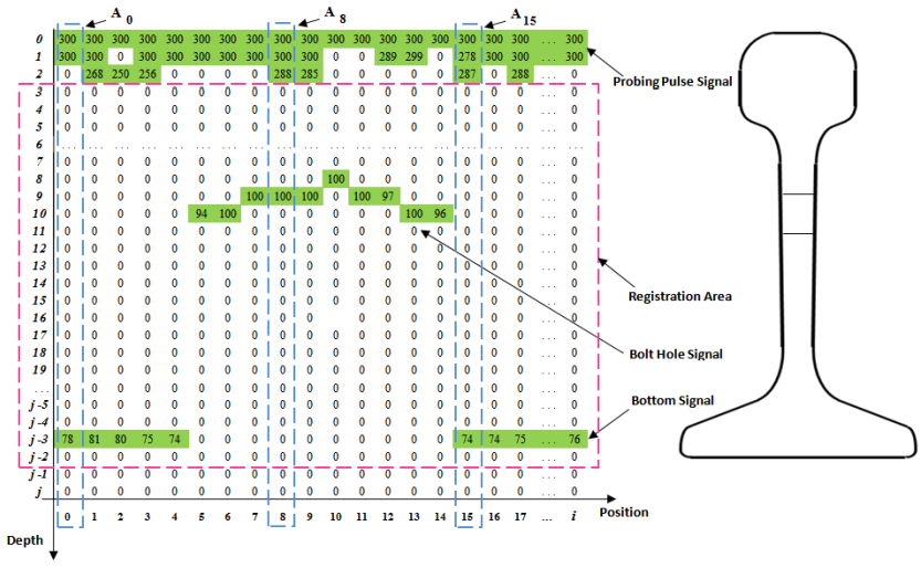
Fig. 2: Fragment of the array with the signals of the bolt hole and the bottom signal.
The graphical representation of the two-dimensional array B in the form of an intensity graph is called «Bright-scan» («B-scan»), Figure 3, while the values of the array are displayed in three dimensions on a plane by using color as the third dimension of the data along the Z-axis.
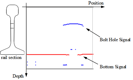
Fig. 3: Fragment of the B-scan of a bolt hole obtained by scanning with a perpendicular input of the probing pulse to the surface of the rail (Avikon-11 equipment).
Formation of a Defectogram
The different reflective properties of defects, their geometry, and their location in the rail require the use of ultrasonic transducers with different angles of input and registration for their detection. Therefore, modern rail flaw detectors use several transducers that are distributed along the length of the flaw detector search system and form a so-called rail section sounding scheme. One of the applied inspection schemes is shown in Figure 4, where the generating and registering transducers of each angle of ultrasonic input are located in the same housing.
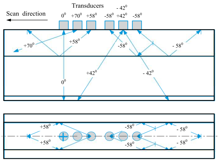
Fig. 4: Example of a scheme for emitting ultrasonic pulses into a rail using six transducers
The formation of B-scan signals for a bolt hole using transducers with central input angles of «+420» (orange), « – 420» (blue), and «00» (green) at three characteristic points (1, 2, 3 positions) along the length of the rail is shown schematically in Figure 5a.
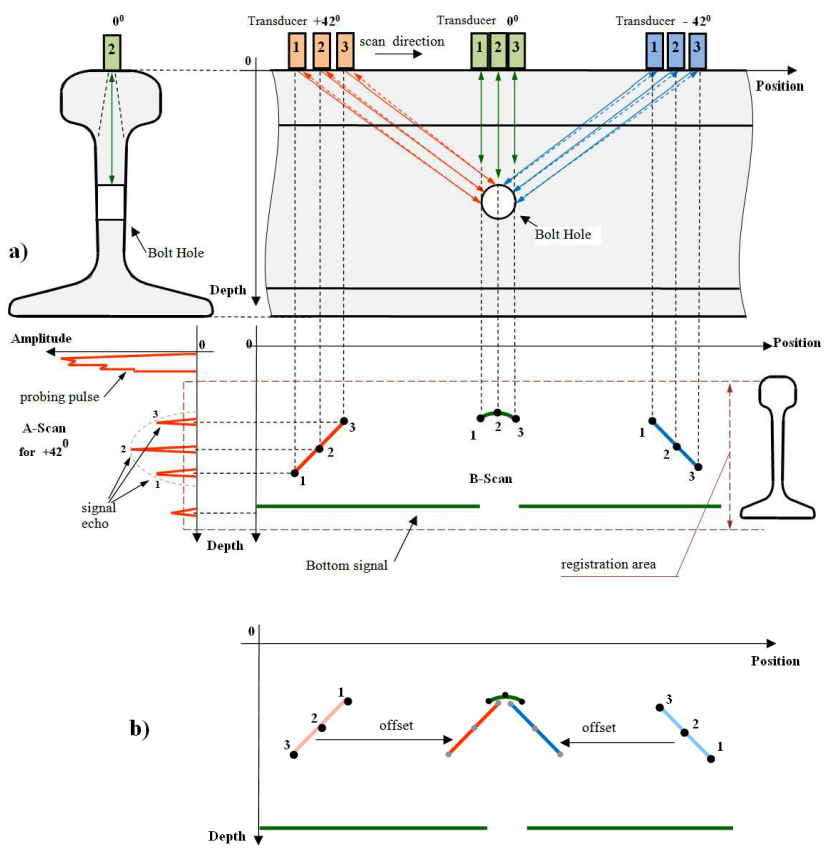
Fig. 5: Signal formation during scanning: a) general view b) correction with offset.
The information channels of a flaw detector correspond to physical sensors (transducers) that are sequentially arranged on the surface of the rail. The set of B-scans for all channels of a flaw detector for each rail, combined into a data file, is called a defectogram (scan). Often, a channel or a set of channels selected for consideration is also called a defectogram.
In most cases, to improve the perception of the defectogram, it is displayed in the mode of reducing to a single section, in which the coordinates of the echo signals for channels with an inclined input of ultrasound are corrected by additionally taking into account the distance of the reflector from the point of input of the probing pulse into the metal of the rail (Figure 5b). In addition, for ease of use and reduction of the graphic appearance of the entire defectogram, a graphical grouping of data channels is performed, one of which is shown in Figure 6.
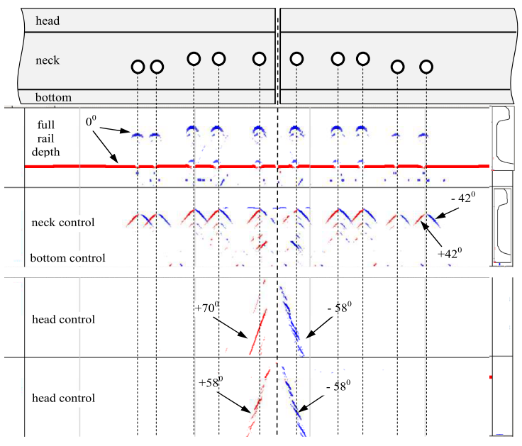
Fig. 6: An example of a section of a defectogram of a bolted rail joint obtained by scanning with ultrasonic equipment Avicon-11.
Decoding Defectograms (Information Feature)
To visually search for defects on the B-scan and A-scan, the cognitive functions of attracted experts — flaw detectors — are used. When ultrasonic scanning of rails, their structural elements and defects have acoustic responses, which are displayed on the defectogram in the form of characteristic graphic images. Each type of defect on the defectogram is visually distinguishable for experts during the data analysis process. The main goal of defectogram analysis is to reliably find and highlight graphic images of defects against the background of possible interference and images of structural elements.
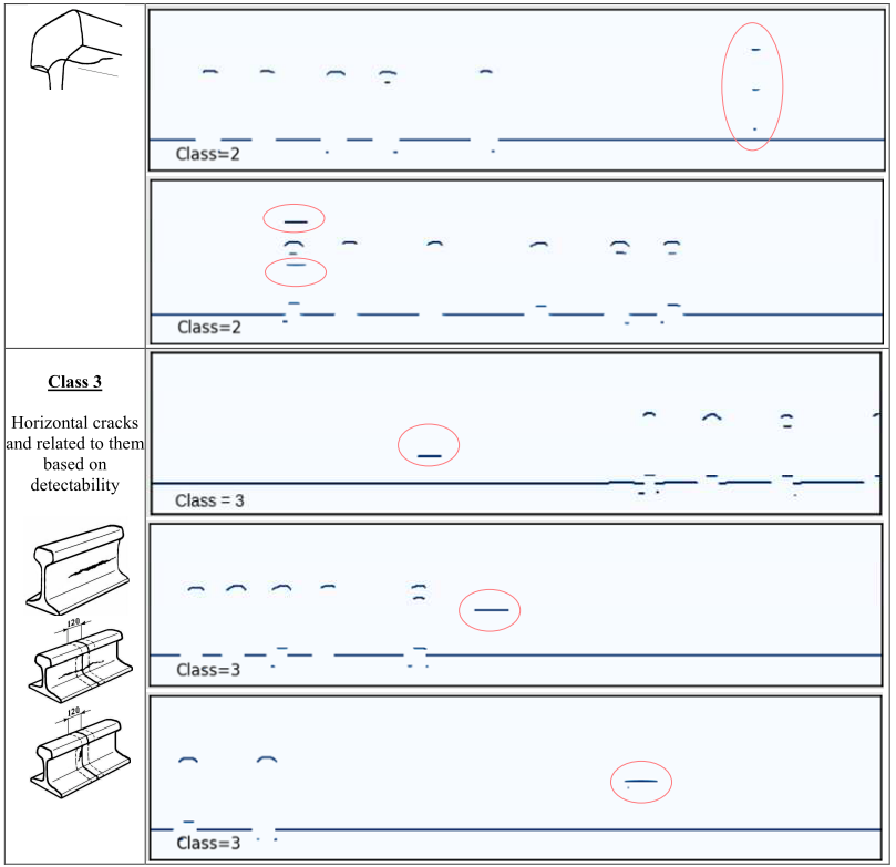
Each measuring channel of the defectogram 00, ±420, ±580, +700 or their combination is designed to detect a specific group of defects. To simplify the task of searching for defects, we will decompose the problem and consider the capabilities of DL algorithms for searching for individual types of defective areas using the defectogram of channel «00» of the Avicon-11 flaw detector. In this case, the types of sites can be divided into four classes based on characteristic information features. Some idea of the diversity of the data set obtained by the Avicon-11 flaw detector can be obtained from Table 1.
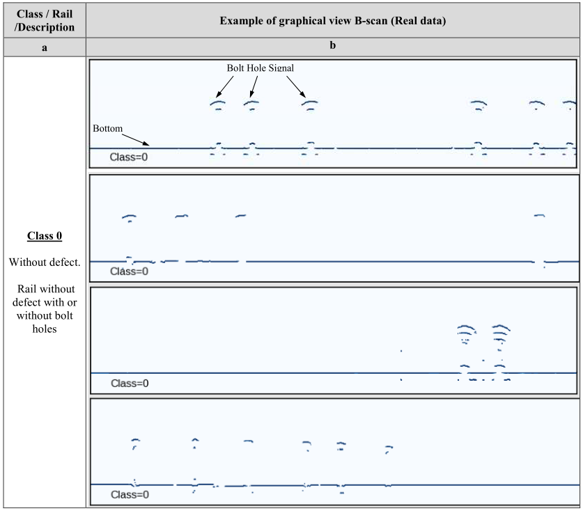
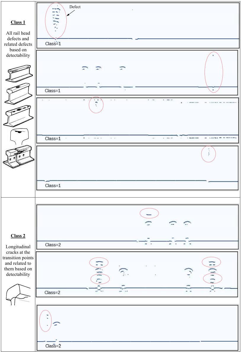
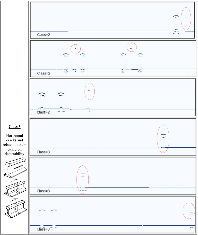
Table 1: Examples of instances (B-scan) for selected classes (real data)
Selection and Implementation of a Classification Algorithm
Despite the fact that in the operation of the railway track, the presence or absence of a defect (binary classification) is decisive, we will quantitatively assess which defective areas have a high probability of being falsely classified as non-defective, which is a dangerous case in rail diagnostics. In this work, the classification task is reduced to an unambiguous multi-class task with four classes.
Data Set Generation
The data set is collected from defectograms obtained by the Avicon-11 flaw detector on several Railroad Test Tracks (RTT) and conventional tracks under various conditions. Each data instance is represented as rectangular “depth × long” data and has the shape (224, 1024), which allows you to fit images of more than six bolt holes along the length of the rail at their bolted joint.
The formation of a data set is difficult due to the lack of a sufficient number of defective areas, so to expand it, we used a displacement along the length of the rail and scanning of the same defect under different conditions and test equipment settings, which allows us to obtain different images of defects (Fig. 7).
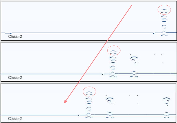
Fig. 7: Example of dataset expansion
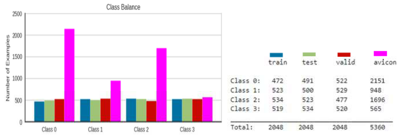
As a result of the specified methodology, the dataset for classes 0, 1, 2, and 3 is 2151, 1043, 1584, and 582, respectively, for a total of 5360 instances. The defect-free class «0» contains 10% (214 instances) of instances without bolt holes, and the remaining 90% (1937 instances) contain from one to six bolt holes. The dataset is named “avicon” and is used only for final testing. This allows us to avoid the problem of class imbalance during training and to obtain a more reliable assessment of the accuracy of the classifier.
For the purposes of training and testing classification models in this work, a synthetic, balanced dataset is used, obtained on the basis of mathematical modeling of models describing the process of reflection and registration of ultrasonic waves from structural reflectors of rails and defects. The application of such a trained model for the classification of real data obtained by a flaw detector during rail diagnostics is demonstrated in Fig. 8.
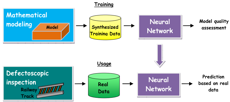
Fig. 8: Application of a neural network trained on model data
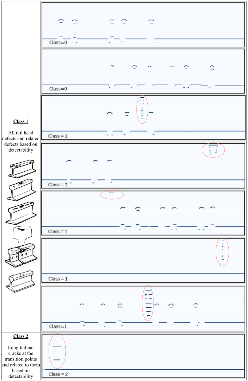
Examples of synthetic instances of the selected classes are presented in Table 2. For more information on the generation of synthetic datasets, please see the works [1-4].
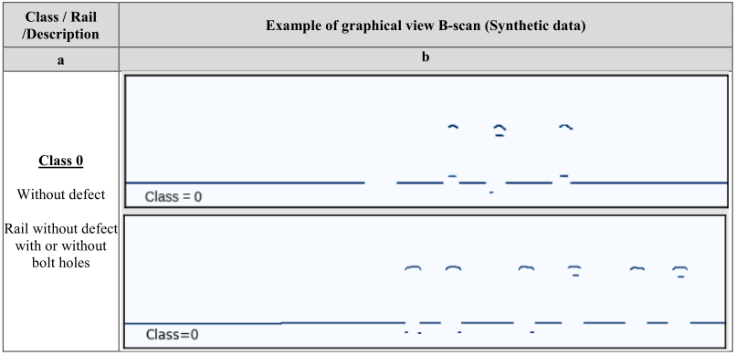
The modeling process allows us to obtain a significant number of instances; we will limit our work to 2048 instances for each of the synthetic sets «train», «valid», «test».
Each instance of data and label is written for each set in the corresponding binary files images.bin and labels.bin (data type «uint8») according to Fig. 9.
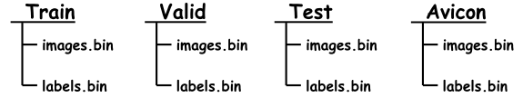
Fig. 9: Distribution of sets by directory
Exploratory Data Analysis
Information on the amount of data, class balance for synthetic sets, and the «avicon» set is presented in Fig. 10.
Analysis of the graphical representation of frames of real data allows us to identify at least one important property of class 3 defects: the images of defects are most difficult to distinguish from the images of bolt holes, especially if they are at the same level as the rail depth, which significantly complicates the classification task.
Each data instance is 224 x 1024 in size, which is large enough for the application of machine learning (ML) algorithms but also causes difficulties in organizing the training process. Each such instance can be considered as data points in a 224*1024 = 229376-dimensional space, which is highly sparse because it contains a large number of zeros. The constructed graph of the integral explainable dispersion of the «train» set as a function of the number of components of the PCA method (Fig. 11) shows that when using 1000 components (330 times smaller than the original size) already 98.5% of the dispersion is explained, which indicates a high level of redundancy in the original data. Such a reduced dataset can be used in ML algorithms, but obtaining it on the entire dataset at the same time causes difficulties; therefore, further in the work, an algorithm based on Deep Learning is considered.
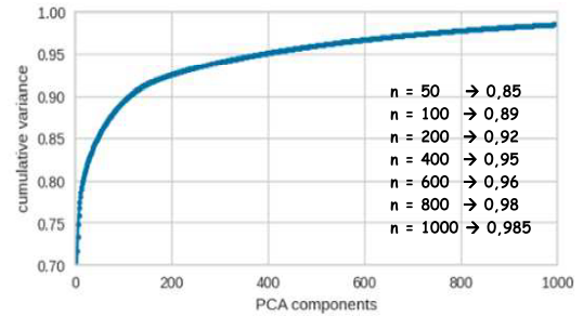
Fig. 11: Graph of the integral explainable dispersion of the data as a function of the number of components of the PCA method for the «train» dataset
Neural Network Architecture
In the work, a DL model in the form of a linear stack of layers is considered (Fig. 12a: the final version of the network). Activation function: relu (rectified linear unit), for the output fully connected layer — normalized exponential softmax function, with the sum of the values of all output neurons equal to one. Loss function: a measure of error in the form of the distance between the probability distributions of actual data and their forecast (cross-entropy). Optimizer: stochastic gradient descent algorithm in the RMSProp modification. Metrics in the training process: accuracy, as a value equal to the ratio of the number of correctly classified objects to the total number of objects.
Network Training
The final version of the network was trained for 50 epochs. The graphs of the changes in the quality indicators «loss» and «accuracy» characterizing the training process (Fig. 12b) converge at the training and validation stages and have low and high values, respectively, which may indicate the absence of the overfitting effect of the model. This fact is also confirmed by the relative equality of the obtained prediction accuracies of the model on the «train» set – 99.61% and the «test» set – 99.02% (Fig. 12b,c). The memory occupied by the network in H5 format is 30 KB. The full code can be found in the GitHub repository at the link [5].
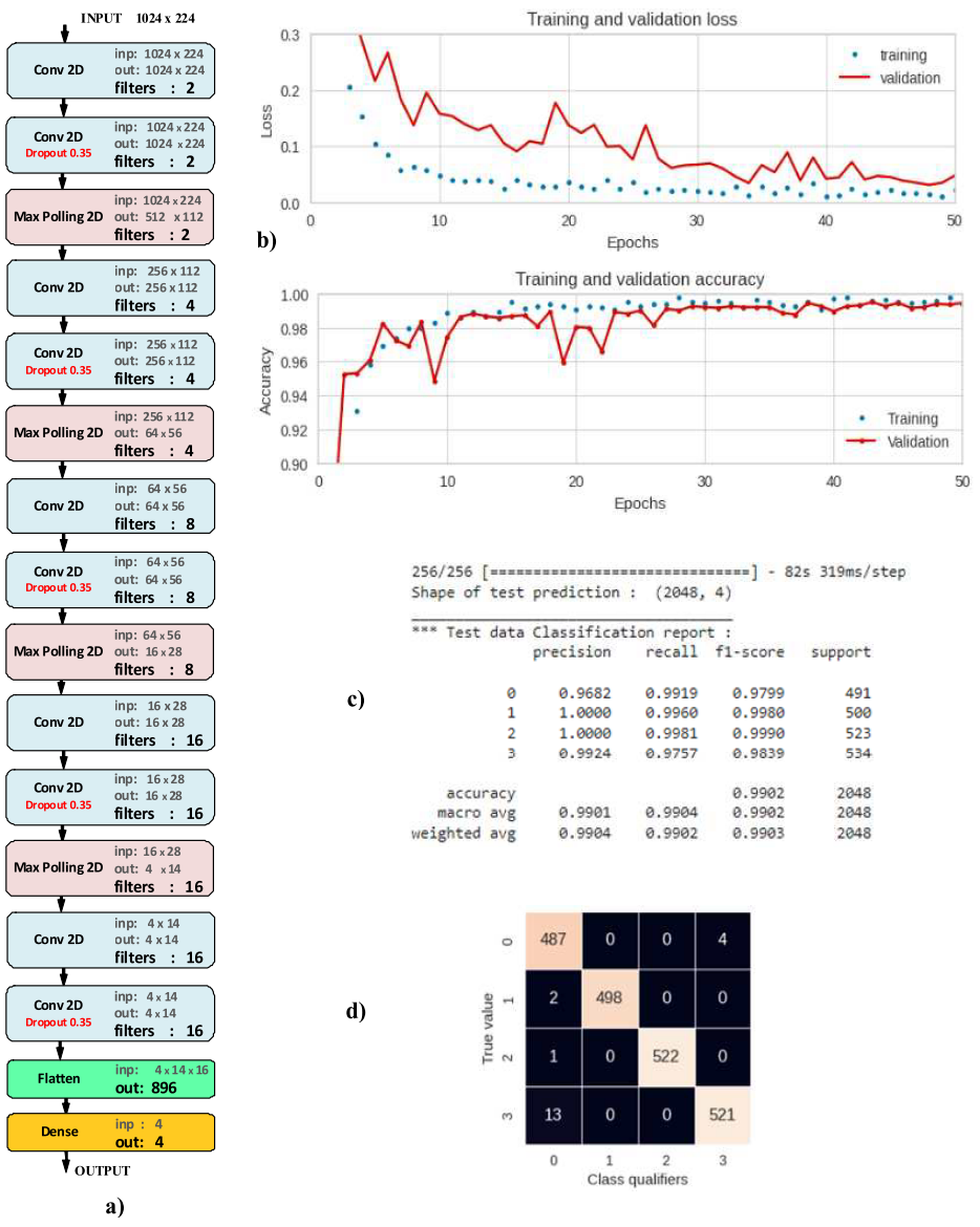
Fig. 12: NN and the results of its training: a) network architecture; b) Change in «Loss» and «Accuracy» during training; c) Classification Report; d) Confusion matrix
The confusion matrix and the classification report are presented in Figure 12d,c. The trained model has high precision and recall scores above 96% for all class classifiers, which also means that there are sufficient information features in the data for classification.
It is important to consider the misclassified samples to understand the operation of the classifier and its changes. According to the confusion matrix, the classifier of class 3 incorrectly recognized four samples of class 0 that have at least one bolt-hole signal similar to the image of a defect of group 3 (an example is shown in Fig. 13a), which may have been the cause of the error.
The class 0 classifier incorrectly recognized two samples of class 1. Both incorrectly recognized defects have a characteristic appearance and are located very close to the upper boundary of the data frame. One of such frames is shown in Fig. 13b.
The class 0 classifier incorrectly recognized one sample of class 2, which is located close enough to the depth of the bolt holes (Fig. 13c).
The class 0 classifier incorrectly recognized 13 samples of class 3, which is located close enough to the depth of the bolt holes (Fig. 13d).
The results of the network tests indicate the difficulty of distinguishing a class 3 defect from bolt holes.
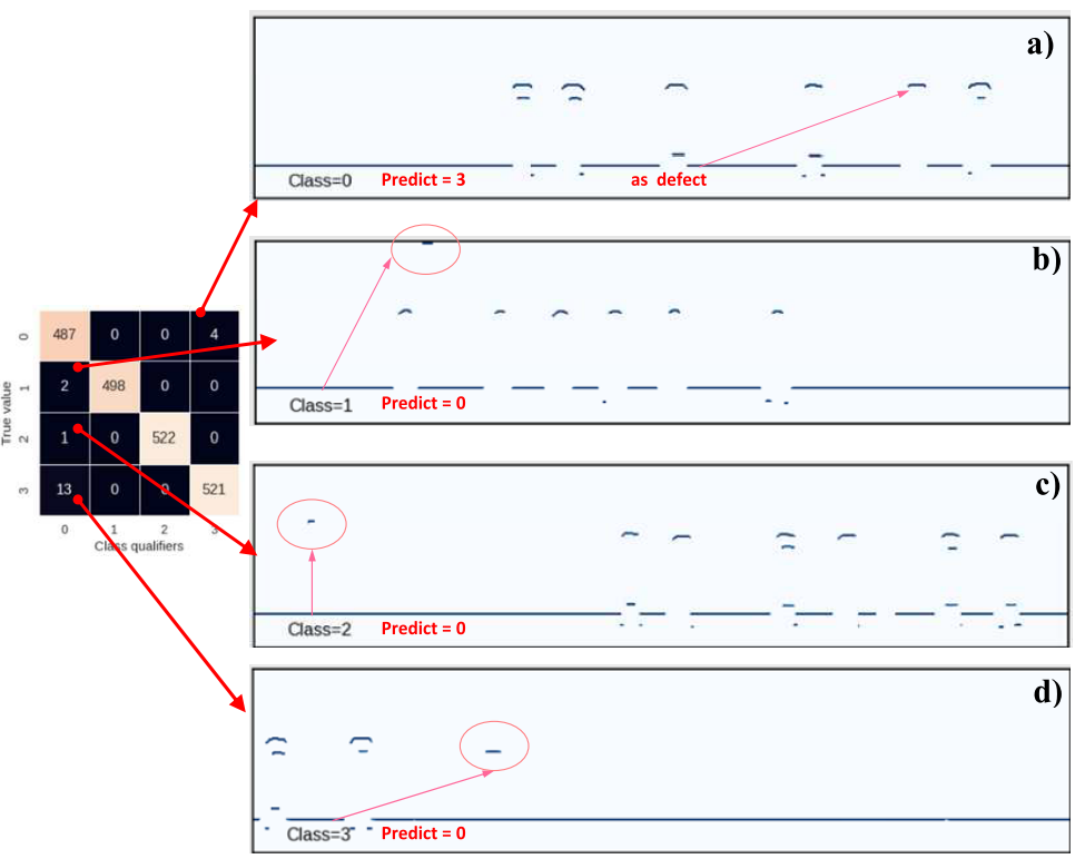
Fig. 13: Characteristic frames of incorrectly classified data
Evaluation of Network Efficiency Using Real Data («Avicon»)
To assess the quality of the work of the trained neural network for recognizing instances of real data obtained by the Avicon-11 flaw detector, modeling was performed on the avicon dataset. The accuracy of the entire network was 90%, which is 9% lower than the prediction accuracy for synthetic data. The resulting confusion matrix and summary report on the quality of the model are presented in Fig. 14. The time required to classify the tagged data makes it possible to estimate the time required to classify 100 km of railway line — 11 s.
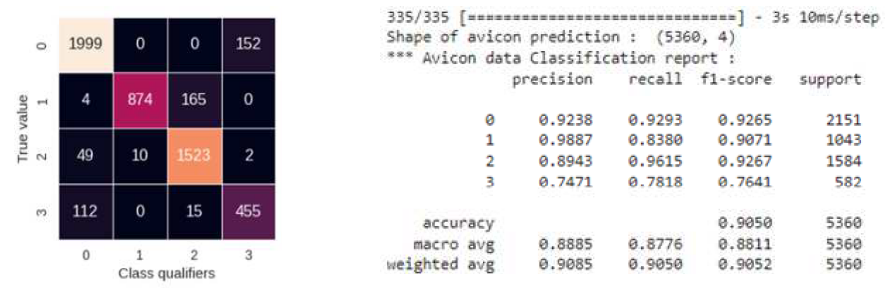
Fig. 14: Summary report on the quality of the model based on the classification of the «avicon» dataset
We will analyze the most important data classification errors. According to the confusion matrix (Fig. 14), four transverse cracks with the weakest response recorded by channel «00» and belonging to class 1 were classified as class 0 (without defect). To improve the recognition of such defects, it is necessary to add additional information features that can be obtained from the inclined channels of the flaw detector, which are the main channels for detecting such types of defects (Fig. 15).
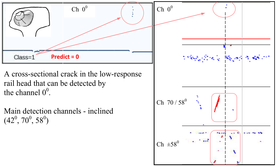
Fig. 15: Typical frames of misclassified data (True = 1, Predict = 0))
The incorrect classification of 49 class 2 defects as non-defective is associated with weak signal responses recorded by the measuring channel «00». One way to improve the classification of such class 2 samples is to consider additional information features from the inclined channels (Ch ±420), as they are the main channels for detecting incorrectly classified defects (Fig. 16).
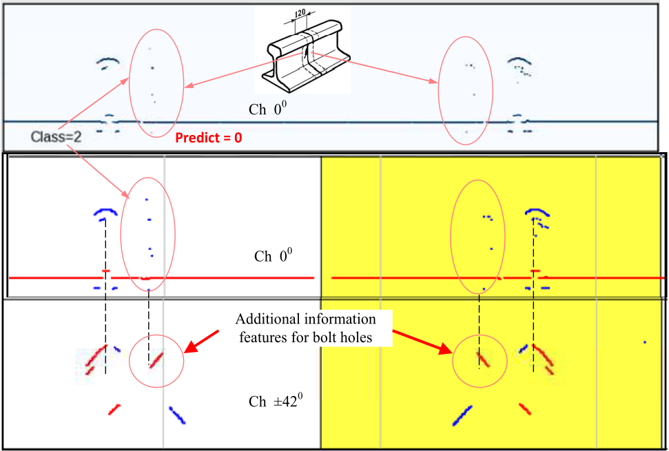
Fig. 16: Typical misclassified data frame of class 2 (True =2, Predict = 0)
The misclassification of 112 class 3 samples to class 0 is associated with data frames where the defect image is:
- Is at the level of bolt holes
- Located closer to the edge of the data frame
- Has a similar pattern to bolt holes
The misclassification of 152 class 0 samples into class 3 samples is due to a similar reason — the similarity of bolt-hole patterns to class 3 defect patterns.
One of the ways to improve the classification of samples of classes 0 and 3 is to consider additional information signs of inclined channels (Ch ±420), since in this case the bolt holes are well distinguished from a defect of class 3 and vice versa (Fig. 17).
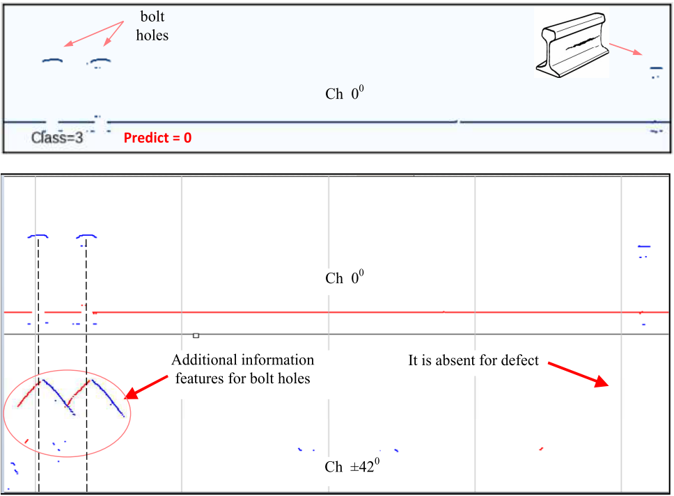
Fig. 17: Typical misclassified data frame of class 3 (True =3, Predict = 0)
The graphical images of defects of classes 1 and 2 are similar, and the assignment of a defect to class 1 or 2 depends on the depth from which the image of the defect begins to be recorded on the defectogram. Defects of class 1 are located in the head of the rail. Defects of class 2 can be recorded starting from the transition zone of the rail from its head to the neck zone. The incorrect classification of 165 defects of class 1 as defects of class 2 is most likely associated with weak defect responses recorded in the head of the rail (Fig. 18).
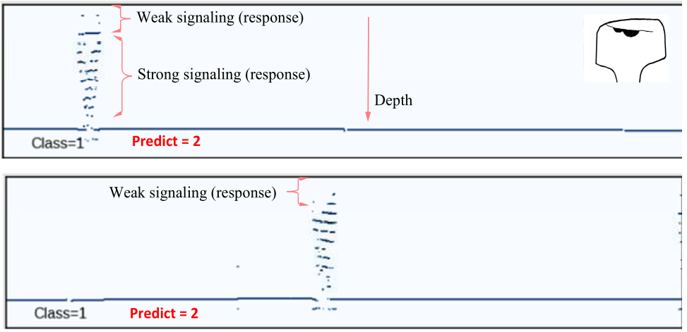
Fig. 18: Typical misclassified data frames of class 1 (True =1, Predict = 2)
Binary Classifier
One of the important tasks of the obtained classifier in its practical use will be the accurate definition of the non-defective class (class 0), which will allow the exclusion of the false assignment of defective samples to non-defective ones. It is possible to reduce the number of false positives for the class 0 classifier by changing the probability cutoff threshold. To evaluate the applicable threshold level of cutoff, the multiclass task was binarized with the isolation of the non-defective state and all defective states, which corresponds to the «one versus rest» strategy (One vs Rest). By default, for binary classification, the threshold value is taken to be 0.5 (50%). With this approach, the binary classifier has an accuracy of 92.28% (Fig. 19).
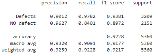
Fig. 19: Qualitative indicators of a binary classifier at a cutoff threshold of 0.5 («avicon» set)
The changes in precision and recall of the binary classifier depending on the changing threshold value are presented in a «precision-recall curve» graph (Fig. 20a). With a threshold value of 0.5, the value of false positives is 161 samples (Fig. 20b). Increasing the threshold value to 0.8, and 0.9 allows to reduce the number of false positives to 70 and 58, respectively, due to an increase in false negatives to 344 and 440 (Fig. 20b).
It can be said that in automatic analysis, increasing the threshold value allows, on the one hand, to reduce the false assignment of defects to the non-defective state and thereby reduce the risk of missing defects. On the other hand, increases the labor intensity of a person during manual analysis of frames with known defects.
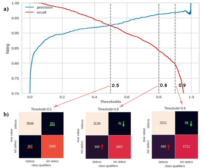
Fig. 20: Influence of the cutoff threshold on the characteristics of a binary classifier: a) precision-recall curve, b) confusion matrix at different cutoff thresholds.
5. Conclusion
- Based on the analysis of the subject area of ultrasonic inspection of rails, information signs of defects were identified, allowing us to identify four classes of rail sections for their classification using machine learning methods.
- A dataset of ultrasonic rail inspection was collected and annotated, which includes 5360 instances.
- Synthetic training, test, and validation datasets were created based on stochastic mathematical modeling of models describing the process of reflection and registration of ultrasonic waves from structural reflectors of rails and defects.
- To solve the problem of unambiguous multi-class classification, a neural network structure based on a convolutional model with an overall accuracy of 99% was trained.
- The effectiveness of using a neural network trained on model data for the recognition of images of real rail defects has been confirmed.
- An estimate of the achievable classification accuracy of 90% has been given using only sections of defectograms of the zero channel of an ultrasonic flaw detector.
- An analysis of the causes of neural network errors has been conducted, and the need for the use of additional information features from defectograms of inclined channels of a flaw detector has been shown.
References
To ensure the safety of rail traffic, non-destructive testing of rails is regularly carried out using various approaches and methods. One of the main approaches to determining the operational condition of railway rails is ultrasonic non-destructive testing. The assessment of the test results depends on the defectoscopist. The need to reduce the workload on humans and improve the efficiency of the process of analyzing ultrasonic testing data makes the task of creating an automated system relevant. The purpose of this work is to evaluate the possibility of creating an effective system for recognizing rail defects from ultrasonic inspection defectograms using ML methods.
Domain Analysis
The railway track consists of rail sections connected together by bolts and welded joints. When a defectoscope device equipped with generating piezoelectric transducers (PZTs) passes along the railway track, ultrasonic pulses are emitted into the rail at a predetermined frequency. The receiving PZTs then register the reflected waves. The detectability of defects by the ultrasonic method is based on the principle of reflection of waves from inhomogeneities in the metal since cracks, including other inhomogeneities, differ in their acoustic resistance from the rest of the metal.
Principle of A-Scan Formation
The registered signal reflected from a bolt hole with a perpendicular input of the probing pulse to the rail surface is presented in Figure 1. The image of such a signal is called «Amplitude scan» or abbreviated «A-scan».
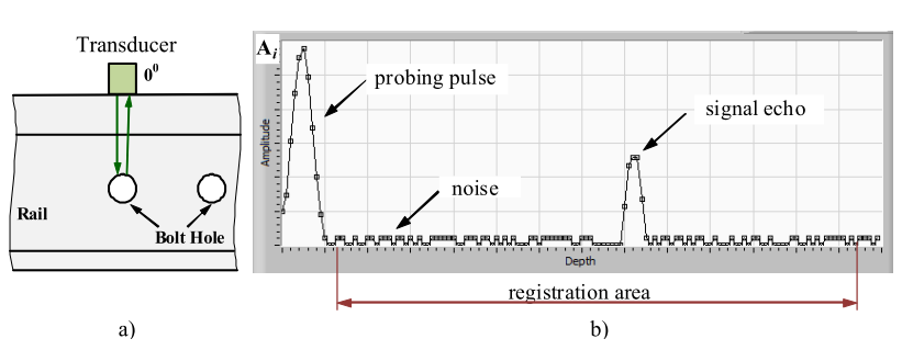
Fig. 1: Presentation of the registered ultrasonic inspection signal on A-scan: a) ultrasound emission and registration process, b) registered signal.
The recorded amplitude of such an echo signal at each i coordinate along the length of the rail can be represented as a vector. Ai = [a1, a2, a3, … , a j ], where aj – is the amplitude of the reflected signal at the j-th depth level of the rail. The depth for each amplitude value aj is calculated based on the registration time and the frequency of the emitted signal.
Principle of B-Scan Formation
The recorded A-scan echo signals at each i inspection point along the length of the rail can be represented as a two-dimensional array. B = [A1, A2, A3, … , Ai] of size (i x j). Figure 2 schematically shows a fragment of array B with the recorded echo signals reflected from a bolt hole with a perpendicular input of the probing pulse to the surface of the rail.
Fig. 2: Fragment of the array with the signals of the bolt hole and the bottom signal.
The graphical representation of the two-dimensional array B in the form of an intensity graph is called «Bright-scan» («B-scan»), Figure 3, while the values of the array are displayed in three dimensions on a plane by using color as the third dimension of the data along the Z-axis.
Fig. 3: Fragment of the B-scan of a bolt hole obtained by scanning with a perpendicular input of the probing pulse to the surface of the rail (Avikon-11 equipment).
Formation of a Defectogram
The different reflective properties of defects, their geometry, and their location in the rail require the use of ultrasonic transducers with different angles of input and registration for their detection. Therefore, modern rail flaw detectors use several transducers that are distributed along the length of the flaw detector search system and form a so-called rail section sounding scheme. One of the applied inspection schemes is shown in Figure 4, where the generating and registering transducers of each angle of ultrasonic input are located in the same housing.
Fig. 4: Example of a scheme for emitting ultrasonic pulses into a rail using six transducers
The formation of B-scan signals for a bolt hole using transducers with central input angles of «+420» (orange), « – 420» (blue), and «00» (green) at three characteristic points (1, 2, 3 positions) along the length of the rail is shown schematically in Figure 5a.
Fig. 5: Signal formation during scanning: a) general view b) correction with offset.
The information channels of a flaw detector correspond to physical sensors (transducers) that are sequentially arranged on the surface of the rail. The set of B-scans for all channels of a flaw detector for each rail, combined into a data file, is called a defectogram (scan). Often, a channel or a set of channels selected for consideration is also called a defectogram.
In most cases, to improve the perception of the defectogram, it is displayed in the mode of reducing to a single section, in which the coordinates of the echo signals for channels with an inclined input of ultrasound are corrected by additionally taking into account the distance of the reflector from the point of input of the probing pulse into the metal of the rail (Figure 5b). In addition, for ease of use and reduction of the graphic appearance of the entire defectogram, a graphical grouping of data channels is performed, one of which is shown in Figure 6.
Fig. 6: An example of a section of a defectogram of a bolted rail joint obtained by scanning with ultrasonic equipment Avicon-11.
Decoding Defectograms (Information Feature)
To visually search for defects on the B-scan and A-scan, the cognitive functions of attracted experts — flaw detectors — are used. When ultrasonic scanning of rails, their structural elements and defects have acoustic responses, which are displayed on the defectogram in the form of characteristic graphic images. Each type of defect on the defectogram is visually distinguishable for experts during the data analysis process. The main goal of defectogram analysis is to reliably find and highlight graphic images of defects against the background of possible interference and images of structural elements.
Each measuring channel of the defectogram 00, ±420, ±580, +700 or their combination is designed to detect a specific group of defects. To simplify the task of searching for defects, we will decompose the problem and consider the capabilities of DL algorithms for searching for individual types of defective areas using the defectogram of channel «00» of the Avicon-11 flaw detector. In this case, the types of sites can be divided into four classes based on characteristic information features. Some idea of the diversity of the data set obtained by the Avicon-11 flaw detector can be obtained from Table 1.
Table 1: Examples of instances (B-scan) for selected classes (real data)
Selection and Implementation of a Classification Algorithm
Despite the fact that in the operation of the railway track, the presence or absence of a defect (binary classification) is decisive, we will quantitatively assess which defective areas have a high probability of being falsely classified as non-defective, which is a dangerous case in rail diagnostics. In this work, the classification task is reduced to an unambiguous multi-class task with four classes.
Data Set Generation
The data set is collected from defectograms obtained by the Avicon-11 flaw detector on several Railroad Test Tracks (RTT) and conventional tracks under various conditions. Each data instance is represented as rectangular “depth × long” data and has the shape (224, 1024), which allows you to fit images of more than six bolt holes along the length of the rail at their bolted joint.
The formation of a data set is difficult due to the lack of a sufficient number of defective areas, so to expand it, we used a displacement along the length of the rail and scanning of the same defect under different conditions and test equipment settings, which allows us to obtain different images of defects (Fig. 7).
Fig. 7: Example of dataset expansion
As a result of the specified methodology, the dataset for classes 0, 1, 2, and 3 is 2151, 1043, 1584, and 582, respectively, for a total of 5360 instances. The defect-free class «0» contains 10% (214 instances) of instances without bolt holes, and the remaining 90% (1937 instances) contain from one to six bolt holes. The dataset is named “avicon” and is used only for final testing. This allows us to avoid the problem of class imbalance during training and to obtain a more reliable assessment of the accuracy of the classifier.
For the purposes of training and testing classification models in this work, a synthetic, balanced dataset is used, obtained on the basis of mathematical modeling of models describing the process of reflection and registration of ultrasonic waves from structural reflectors of rails and defects. The application of such a trained model for the classification of real data obtained by a flaw detector during rail diagnostics is demonstrated in Fig. 8.
Fig. 8: Application of a neural network trained on model data
Examples of synthetic instances of the selected classes are presented in Table 2. For more information on the generation of synthetic datasets, please see the works [1-4].
The modeling process allows us to obtain a significant number of instances; we will limit our work to 2048 instances for each of the synthetic sets «train», «valid», «test».
Each instance of data and label is written for each set in the corresponding binary files images.bin and labels.bin (data type «uint8») according to Fig. 9.
Fig. 9: Distribution of sets by directory
Exploratory Data Analysis
Information on the amount of data, class balance for synthetic sets, and the «avicon» set is presented in Fig. 10.
Analysis of the graphical representation of frames of real data allows us to identify at least one important property of class 3 defects: the images of defects are most difficult to distinguish from the images of bolt holes, especially if they are at the same level as the rail depth, which significantly complicates the classification task.
Each data instance is 224 x 1024 in size, which is large enough for the application of machine learning (ML) algorithms but also causes difficulties in organizing the training process. Each such instance can be considered as data points in a 224*1024 = 229376-dimensional space, which is highly sparse because it contains a large number of zeros. The constructed graph of the integral explainable dispersion of the «train» set as a function of the number of components of the PCA method (Fig. 11) shows that when using 1000 components (330 times smaller than the original size) already 98.5% of the dispersion is explained, which indicates a high level of redundancy in the original data. Such a reduced dataset can be used in ML algorithms, but obtaining it on the entire dataset at the same time causes difficulties; therefore, further in the work, an algorithm based on Deep Learning is considered.
Fig. 11: Graph of the integral explainable dispersion of the data as a function of the number of components of the PCA method for the «train» dataset
Neural Network Architecture
In the work, a DL model in the form of a linear stack of layers is considered (Fig. 12a: the final version of the network). Activation function: relu (rectified linear unit), for the output fully connected layer — normalized exponential softmax function, with the sum of the values of all output neurons equal to one. Loss function: a measure of error in the form of the distance between the probability distributions of actual data and their forecast (cross-entropy). Optimizer: stochastic gradient descent algorithm in the RMSProp modification. Metrics in the training process: accuracy, as a value equal to the ratio of the number of correctly classified objects to the total number of objects.
Network Training
The final version of the network was trained for 50 epochs. The graphs of the changes in the quality indicators «loss» and «accuracy» characterizing the training process (Fig. 12b) converge at the training and validation stages and have low and high values, respectively, which may indicate the absence of the overfitting effect of the model. This fact is also confirmed by the relative equality of the obtained prediction accuracies of the model on the «train» set – 99.61% and the «test» set – 99.02% (Fig. 12b,c). The memory occupied by the network in H5 format is 30 KB. The full code can be found in the GitHub repository at the link [5].
Fig. 12: NN and the results of its training: a) network architecture; b) Change in «Loss» and «Accuracy» during training; c) Classification Report; d) Confusion matrix
The confusion matrix and the classification report are presented in Figure 12d,c. The trained model has high precision and recall scores above 96% for all class classifiers, which also means that there are sufficient information features in the data for classification.
It is important to consider the misclassified samples to understand the operation of the classifier and its changes. According to the confusion matrix, the classifier of class 3 incorrectly recognized four samples of class 0 that have at least one bolt-hole signal similar to the image of a defect of group 3 (an example is shown in Fig. 13a), which may have been the cause of the error.
The class 0 classifier incorrectly recognized two samples of class 1. Both incorrectly recognized defects have a characteristic appearance and are located very close to the upper boundary of the data frame. One of such frames is shown in Fig. 13b.
The class 0 classifier incorrectly recognized one sample of class 2, which is located close enough to the depth of the bolt holes (Fig. 13c).
The class 0 classifier incorrectly recognized 13 samples of class 3, which is located close enough to the depth of the bolt holes (Fig. 13d).
The results of the network tests indicate the difficulty of distinguishing a class 3 defect from bolt holes.
Fig. 13: Characteristic frames of incorrectly classified data
Evaluation of Network Efficiency Using Real Data («Avicon»)
To assess the quality of the work of the trained neural network for recognizing instances of real data obtained by the Avicon-11 flaw detector, modeling was performed on the avicon dataset. The accuracy of the entire network was 90%, which is 9% lower than the prediction accuracy for synthetic data. The resulting confusion matrix and summary report on the quality of the model are presented in Fig. 14. The time required to classify the tagged data makes it possible to estimate the time required to classify 100 km of railway line — 11 s.
Fig. 14: Summary report on the quality of the model based on the classification of the «avicon» dataset
We will analyze the most important data classification errors. According to the confusion matrix (Fig. 14), four transverse cracks with the weakest response recorded by channel «00» and belonging to class 1 were classified as class 0 (without defect). To improve the recognition of such defects, it is necessary to add additional information features that can be obtained from the inclined channels of the flaw detector, which are the main channels for detecting such types of defects (Fig. 15).
Fig. 15: Typical frames of misclassified data (True = 1, Predict = 0))
The incorrect classification of 49 class 2 defects as non-defective is associated with weak signal responses recorded by the measuring channel «00». One way to improve the classification of such class 2 samples is to consider additional information features from the inclined channels (Ch ±420), as they are the main channels for detecting incorrectly classified defects (Fig. 16).
Fig. 16: Typical misclassified data frame of class 2 (True =2, Predict = 0)
The misclassification of 112 class 3 samples to class 0 is associated with data frames where the defect image is:
- Is at the level of bolt holes
- Located closer to the edge of the data frame
- Has a similar pattern to bolt holes
The misclassification of 152 class 0 samples into class 3 samples is due to a similar reason — the similarity of bolt-hole patterns to class 3 defect patterns.
One of the ways to improve the classification of samples of classes 0 and 3 is to consider additional information signs of inclined channels (Ch ±420), since in this case the bolt holes are well distinguished from a defect of class 3 and vice versa (Fig. 17).
Fig. 17: Typical misclassified data frame of class 3 (True =3, Predict = 0)
The graphical images of defects of classes 1 and 2 are similar, and the assignment of a defect to class 1 or 2 depends on the depth from which the image of the defect begins to be recorded on the defectogram. Defects of class 1 are located in the head of the rail. Defects of class 2 can be recorded starting from the transition zone of the rail from its head to the neck zone. The incorrect classification of 165 defects of class 1 as defects of class 2 is most likely associated with weak defect responses recorded in the head of the rail (Fig. 18).
Fig. 18: Typical misclassified data frames of class 1 (True =1, Predict = 2)
Binary Classifier
One of the important tasks of the obtained classifier in its practical use will be the accurate definition of the non-defective class (class 0), which will allow the exclusion of the false assignment of defective samples to non-defective ones. It is possible to reduce the number of false positives for the class 0 classifier by changing the probability cutoff threshold. To evaluate the applicable threshold level of cutoff, the multiclass task was binarized with the isolation of the non-defective state and all defective states, which corresponds to the «one versus rest» strategy (One vs Rest). By default, for binary classification, the threshold value is taken to be 0.5 (50%). With this approach, the binary classifier has an accuracy of 92.28% (Fig. 19).
Fig. 19: Qualitative indicators of a binary classifier at a cutoff threshold of 0.5 («avicon» set)
The changes in precision and recall of the binary classifier depending on the changing threshold value are presented in a «precision-recall curve» graph (Fig. 20a). With a threshold value of 0.5, the value of false positives is 161 samples (Fig. 20b). Increasing the threshold value to 0.8, and 0.9 allows to reduce the number of false positives to 70 and 58, respectively, due to an increase in false negatives to 344 and 440 (Fig. 20b).
It can be said that in automatic analysis, increasing the threshold value allows, on the one hand, to reduce the false assignment of defects to the non-defective state and thereby reduce the risk of missing defects. On the other hand, increases the labor intensity of a person during manual analysis of frames with known defects.
Fig. 20: Influence of the cutoff threshold on the characteristics of a binary classifier: a) precision-recall curve, b) confusion matrix at different cutoff thresholds.
5. Conclusion
- Based on the analysis of the subject area of ultrasonic inspection of rails, information signs of defects were identified, allowing us to identify four classes of rail sections for their classification using machine learning methods.
- A dataset of ultrasonic rail inspection was collected and annotated, which includes 5360 instances.
- Synthetic training, test, and validation datasets were created based on stochastic mathematical modeling of models describing the process of reflection and registration of ultrasonic waves from structural reflectors of rails and defects.
- To solve the problem of unambiguous multi-class classification, a neural network structure based on a convolutional model with an overall accuracy of 99% was trained.
- The effectiveness of using a neural network trained on model data for the recognition of images of real rail defects has been confirmed.
- An estimate of the achievable classification accuracy of 90% has been given using only sections of defectograms of the zero channel of an ultrasonic flaw detector.
- An analysis of the causes of neural network errors has been conducted, and the need for the use of additional information features from defectograms of inclined channels of a flaw detector has been shown.
References
Denial of responsibility! Techno Blender is an automatic aggregator of the all world’s media. In each content, the hyperlink to the primary source is specified. All trademarks belong to their rightful owners, all materials to their authors. If you are the owner of the content and do not want us to publish your materials, please contact us by email – [email protected]. The content will be deleted within 24 hours.