
Solving Autocorrelation Problems in General Linear Model on a Real-World Application
Delving into one of the most common nightmares for data scientists
Introduction
One of the biggest problems in linear regression is autocorrelated residuals. In this context, this article revisits linear regression, delves into the Cochrane–Orcutt procedure as a way to solve this problem, and explores a real-world application in fMRI brain activation analysis.
General Linear Model (GLM) revisited
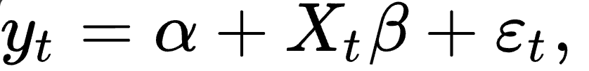
Linear regression is probably one of the most important tools for any data scientist. However, it's common to see many misconceptions being made, especially in the context of time series. Therefore, let's invest some time revisiting the concept. The primary goal of a GLM in time series analysis is to model the relationship between variables over a sequence of time points. Where Y is the target data, X is the feature data, B and A the coefficients to estimate and Ɛ is the Gaussian error.

The index refers to the time evolution of the data. Writing in a more compact form:

by the author.
The estimation of parameters is done through ordinary least squares (OLS), which assumes that the errors, or residuals, between the observed values and the values predicted by the model, are independent and identically distributed (i.i.d).
This means that the residuals must be non-autocorrelated to ensure the right estimation of the coefficients, the validity of the model, and the accuracy of predictions.
Autocorrelation
Autocorrelation refers to the correlation between observations within a time series. We can understand it as how each data point is related to lagged data points in a sequence.
Autocorrelation functions (ACF) are used to detect autocorrelation. These methods measure the correlation between a data point and its lagged values (t = 1,2,…,40), revealing if data points are related to preceding or following values. ACF plots (Figure 1) display correlation coefficients at different lags, indicating the strength of autocorrelation, and the statistical significance over the shade region.
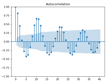
If the coefficients for certain lags significantly differ from zero, it suggests the presence of autocorrelation.
Autocorrelation in the residuals
Autocorrelation in the residuals suggests that there’s a relationship or dependency between current and past errors in the time series. This correlation pattern indicates that the errors are not random and may be influenced by factors not accounted for in the model. For example, autocorrelation can lead to biased parameter estimates, especially in the variance, affecting the understanding of the relationships between variables. This results in invalid inferences drawn from the model, leading to misleading conclusions about relationships between variables. Moreover, it results in inefficient predictions, which means the model is not capturing correct information.
Cochrane–Orcutt procedure
The Cochrane–Orcutt procedure is a method famous in econometrics and in a variety of areas to address issues of autocorrelation in a time series through a linear model for serial correlation in the error term [1,2]. We already know that this violates one of the assumptions of ordinary least squares (OLS) regression, which assumes that the errors (residuals) are uncorrelated [1]. Later in the article, we're going to use the procedure to remove autocorrelation and check how biased the coefficients are.
The Cochrane–Orcutt procedure goes as follows:
- 1. Initial OLS Regression: Start with an initial regression analysis using ordinary least squares (OLS) to estimate the model parameters.
- 2. Residual Calculation: Calculate the residuals from the initial regression.
- 3. Test for Autocorrelation: Examine the residuals for the presence of autocorrelation using ACF plots or tests such as the Durbin-Watson test. If the autocorrelation is not significant, there is no need to follow the procedure.
- 4. Transformation: The estimated model is transformed by differencing the dependent and independent variables to remove autocorrelation. The idea here is to make the residuals closer to being uncorrelated.

- 5. Regress the Transformed Model: Perform a new regression analysis with the transformed model and compute new residuals.
- 6. Check for Autocorrelation: Test the new residuals for autocorrelation again. If autocorrelation remains, go back to step 4 and transform the model further until the residuals show no significant autocorrelation.
Final Model Estimation: Once the residuals exhibit no significant autocorrelation, use the final model and coefficients derived from the Cochrane-Orcutt procedure for making inferences and drawing conclusions!
Real-world application: Functional Magnetic Resonance Imaging (fMRI) analysis
A brief introduction to fMRI
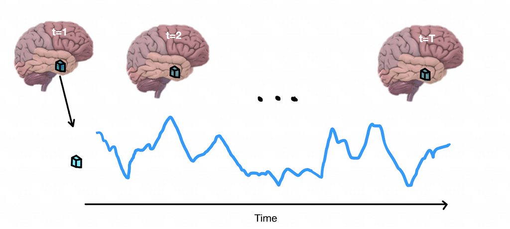
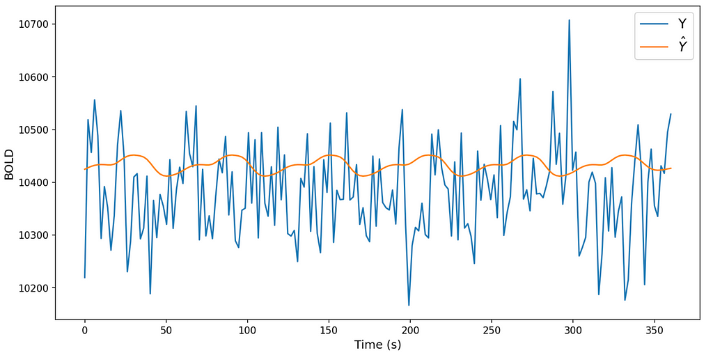
Functional Magnetic Resonance Imaging (fMRI) is a neuroimaging technique that measures and maps brain activity by detecting changes in blood flow. It relies on the principle that neural activity is associated with increased blood flow and oxygenation. In fMRI, when a brain region becomes active, it triggers a hemodynamic response, leading to changes in blood oxygen level-dependent (BOLD) signals. fMRI data typically consists of 3D images representing the brain activation at different time points, therefore each volume (voxel) of the brain has its own time series (Figure 2).
The General Linear Model (GLM)
The GLM assumes that the measured fMRI signal is a linear combination of different factors (features), such as task information mixed with the expected response of neural activity known as the Hemodynamic Response Function (HRF). For simplicity, we're going to ignore the nature of the HRF and just assume that it's an important feature.
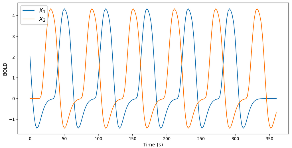
To understand the impact of the tasks on the resulting BOLD signal y (dependent variable), we're going to use a GLM. This translates to checking the effect through statistically significant coefficients associated with the task information. Hence, X1 and X2 (independent variables) are information about the task that was executed by the participant through the data collection convolved with the HRF (Figure 3).

Application on real data
In order to check this Real-World application, we will use data collected by Prof. João Sato at the Federal University of ABC, which is available on GitHub. The independent variable fmri_data contains data from one voxel (a single time series), but we could do it for every voxel in the brain. The dependent variables that contain the task information are cong and incong. The explanations of these variables are out of the scope of this article.
#Reading data
fmri_img = nib.load('/Users/rodrigo/Medium/GLM_Orcutt/Stroop.nii')
cong = np.loadtxt('/Users/rodrigo/Medium/GLM_Orcutt/congruent.txt')
incong = np.loadtxt('/Users/rodrigo/Medium/GLM_Orcutt/incongruent.txt')

#Get the series from each voxel
fmri_data = fmri_img.get_fdata()

#HRF function
HRF = glover(.5)

#Convolution of task data with HRF
conv_cong = np.convolve(cong.ravel(), HRF.ravel(), mode='same')
conv_incong = np.convolve(incong.ravel(), HRF.ravel(), mode='same')
Visualising the task information variables (features).
Fitting GLM
Using Ordinary Least Square to fit the model and estimate the model parameters, we get to
import statsmodels.api as sm
#Selecting one voxel (time series)
y = fmri_data[20,30,30]
x = np.array([conv_incong, conv_cong]).T
#add constant to predictor variables
x = sm.add_constant(x)
#fit linear regression model
model = sm.OLS(y,x).fit()
#view model summary
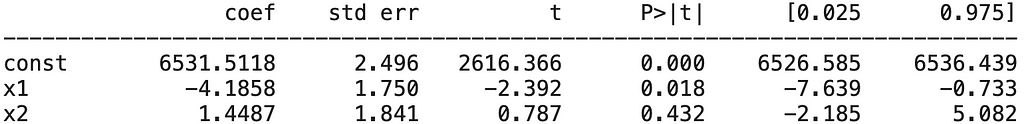
print(model.summary())
params = model.params
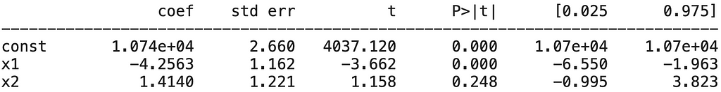
It's possible to see that coefficient X1 is statistically significant, once P > |t| is less than 0.05. That could mean that the task indeed impact the BOLD signal. But before using these parameters to do inference, it’s essential to check if the residuals, which means y minus prediction, are not autocorrelated in any lag. Otherwise, our estimate is biased.
Checking residuals auto-correlation
As already discussed the ACF plot is a good way to check autocorrelation in the series.
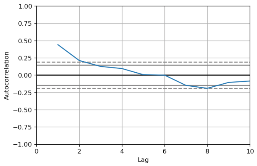
Looking at the ACF plot it’s possible to detect a high autocorrelation at lag 1. Therefore, this linear model is biased and it’s important to fix this problem.
Cochrane-Orcutt to solve autocorrelation in residuals
The Cochrane-Orcutt procedure is widely used in fMRI data analysis to solve this kind of problem [2]. In this specific case, the lag 1 autocorrelation in the residuals is significant, therefore, we can use the Cochrane–Orcutt formula for the autoregressive term AR(1).
# LAG 0
yt = y[2:180]
# LAG 1
yt1 = y[1:179]

# calculate correlation coef. for lag 1
rho= np.corrcoef(yt,yt1)[0,1]

# Cochrane-Orcutt equation
Y2= yt - rho*yt1
X2 = x[2:180,1:] - rho*x[1:179,1:]
Fitting the transformed Model
Fitting the model again but after the Cochrane-Orcutt correction.
import statsmodels.api as sm

#add constant to predictor variables
X2 = sm.add_constant(X2)

#fit linear regression model
model = sm.OLS(Y2,X2).fit()

#view model summary
print(model.summary())
params = model.params
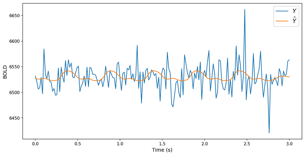
Now the coefficient X1 is not statistically significant anymore, discarding the hypothesis that the task impact the BOLD signal. The parameters standard error estimate changed significantly, which indicates the high impact of autocorrelation in the residuals to the estimation
Checking for autocorrelation again
This makes sense since it's possible to show that the variance is always biased when there is autocorrelation [1].
Now the autocorrelation of the residuals was removed and the estimate is not biased anymore. If we had ignored the autocorrelation in the residuals, we could consider the coefficient significant. However, after removing the autocorrelation, turns out that the parameter is not significant, avoiding a spurious inference that the task is indeed related to signal.
Conclusions
Autocorrelation in the residuals of a General Linear Model can lead to biased estimates, inefficient predictions, and invalid inferences. The application of the Cochrane–Orcutt procedure to real-world fMRI data demonstrates its effectiveness in removing autocorrelation from residuals and avoiding false conclusions, ensuring the reliability of model parameters and the accuracy of inferences drawn from the analysis.
Remarks
Cochrane-Orcutt is just one method to solve autocorrelation in the residuals. However, there are other to address this problem such as Hildreth-Lu Procedure and First Differences Procedure [1].
Acknowledgement
This project was inspired by Prof. João Ricardo Sato.
The notebook for this article is available here.
References
[1] Applied Regression Modeling, Iain Pardoe. Wileyl. 2023. https://online.stat.psu.edu/stat462/node/189/
[2] Sato JR, Takahashi DY, Cardoso EF, Martin Mda G, Amaro Júnior E, Morettin PA. Intervention models in functional connectivity identification applied to FMRI. Int J Biomed Imaging. 2006;2006:27483. doi:10.1155/IJBI/2006/27483
Solving Autocorrelation Problems in General Linear Model on a Real-World Application was originally published in Towards Data Science on Medium, where people are continuing the conversation by highlighting and responding to this story.
Delving into one of the most common nightmares for data scientists
Introduction
One of the biggest problems in linear regression is autocorrelated residuals. In this context, this article revisits linear regression, delves into the Cochrane–Orcutt procedure as a way to solve this problem, and explores a real-world application in fMRI brain activation analysis.

General Linear Model (GLM) revisited
Linear regression is probably one of the most important tools for any data scientist. However, it's common to see many misconceptions being made, especially in the context of time series. Therefore, let's invest some time revisiting the concept. The primary goal of a GLM in time series analysis is to model the relationship between variables over a sequence of time points. Where Y is the target data, X is the feature data, B and A the coefficients to estimate and Ɛ is the Gaussian error.
The index refers to the time evolution of the data. Writing in a more compact form:
by the author.
The estimation of parameters is done through ordinary least squares (OLS), which assumes that the errors, or residuals, between the observed values and the values predicted by the model, are independent and identically distributed (i.i.d).
This means that the residuals must be non-autocorrelated to ensure the right estimation of the coefficients, the validity of the model, and the accuracy of predictions.
Autocorrelation
Autocorrelation refers to the correlation between observations within a time series. We can understand it as how each data point is related to lagged data points in a sequence.
Autocorrelation functions (ACF) are used to detect autocorrelation. These methods measure the correlation between a data point and its lagged values (t = 1,2,…,40), revealing if data points are related to preceding or following values. ACF plots (Figure 1) display correlation coefficients at different lags, indicating the strength of autocorrelation, and the statistical significance over the shade region.
If the coefficients for certain lags significantly differ from zero, it suggests the presence of autocorrelation.
Autocorrelation in the residuals
Autocorrelation in the residuals suggests that there’s a relationship or dependency between current and past errors in the time series. This correlation pattern indicates that the errors are not random and may be influenced by factors not accounted for in the model. For example, autocorrelation can lead to biased parameter estimates, especially in the variance, affecting the understanding of the relationships between variables. This results in invalid inferences drawn from the model, leading to misleading conclusions about relationships between variables. Moreover, it results in inefficient predictions, which means the model is not capturing correct information.
Cochrane–Orcutt procedure
The Cochrane–Orcutt procedure is a method famous in econometrics and in a variety of areas to address issues of autocorrelation in a time series through a linear model for serial correlation in the error term [1,2]. We already know that this violates one of the assumptions of ordinary least squares (OLS) regression, which assumes that the errors (residuals) are uncorrelated [1]. Later in the article, we're going to use the procedure to remove autocorrelation and check how biased the coefficients are.
The Cochrane–Orcutt procedure goes as follows:
- 1. Initial OLS Regression: Start with an initial regression analysis using ordinary least squares (OLS) to estimate the model parameters.
- 2. Residual Calculation: Calculate the residuals from the initial regression.
- 3. Test for Autocorrelation: Examine the residuals for the presence of autocorrelation using ACF plots or tests such as the Durbin-Watson test. If the autocorrelation is not significant, there is no need to follow the procedure.
- 4. Transformation: The estimated model is transformed by differencing the dependent and independent variables to remove autocorrelation. The idea here is to make the residuals closer to being uncorrelated.
- 5. Regress the Transformed Model: Perform a new regression analysis with the transformed model and compute new residuals.
- 6. Check for Autocorrelation: Test the new residuals for autocorrelation again. If autocorrelation remains, go back to step 4 and transform the model further until the residuals show no significant autocorrelation.
Final Model Estimation: Once the residuals exhibit no significant autocorrelation, use the final model and coefficients derived from the Cochrane-Orcutt procedure for making inferences and drawing conclusions!
Real-world application: Functional Magnetic Resonance Imaging (fMRI) analysis
A brief introduction to fMRI
Functional Magnetic Resonance Imaging (fMRI) is a neuroimaging technique that measures and maps brain activity by detecting changes in blood flow. It relies on the principle that neural activity is associated with increased blood flow and oxygenation. In fMRI, when a brain region becomes active, it triggers a hemodynamic response, leading to changes in blood oxygen level-dependent (BOLD) signals. fMRI data typically consists of 3D images representing the brain activation at different time points, therefore each volume (voxel) of the brain has its own time series (Figure 2).
The General Linear Model (GLM)
The GLM assumes that the measured fMRI signal is a linear combination of different factors (features), such as task information mixed with the expected response of neural activity known as the Hemodynamic Response Function (HRF). For simplicity, we're going to ignore the nature of the HRF and just assume that it's an important feature.
To understand the impact of the tasks on the resulting BOLD signal y (dependent variable), we're going to use a GLM. This translates to checking the effect through statistically significant coefficients associated with the task information. Hence, X1 and X2 (independent variables) are information about the task that was executed by the participant through the data collection convolved with the HRF (Figure 3).
Application on real data
In order to check this Real-World application, we will use data collected by Prof. João Sato at the Federal University of ABC, which is available on GitHub. The independent variable fmri_data contains data from one voxel (a single time series), but we could do it for every voxel in the brain. The dependent variables that contain the task information are cong and incong. The explanations of these variables are out of the scope of this article.
#Reading data
fmri_img = nib.load('/Users/rodrigo/Medium/GLM_Orcutt/Stroop.nii')
cong = np.loadtxt('/Users/rodrigo/Medium/GLM_Orcutt/congruent.txt')
incong = np.loadtxt('/Users/rodrigo/Medium/GLM_Orcutt/incongruent.txt')

#Get the series from each voxel
fmri_data = fmri_img.get_fdata()

#HRF function
HRF = glover(.5)

#Convolution of task data with HRF
conv_cong = np.convolve(cong.ravel(), HRF.ravel(), mode='same')
conv_incong = np.convolve(incong.ravel(), HRF.ravel(), mode='same')
Visualising the task information variables (features).
Fitting GLM
Using Ordinary Least Square to fit the model and estimate the model parameters, we get to
import statsmodels.api as sm

#Selecting one voxel (time series)
y = fmri_data[20,30,30]
x = np.array([conv_incong, conv_cong]).T

#add constant to predictor variables
x = sm.add_constant(x)

#fit linear regression model
model = sm.OLS(y,x).fit()

#view model summary
print(model.summary())
params = model.params
It's possible to see that coefficient X1 is statistically significant, once P > |t| is less than 0.05. That could mean that the task indeed impact the BOLD signal. But before using these parameters to do inference, it’s essential to check if the residuals, which means y minus prediction, are not autocorrelated in any lag. Otherwise, our estimate is biased.
Checking residuals auto-correlation
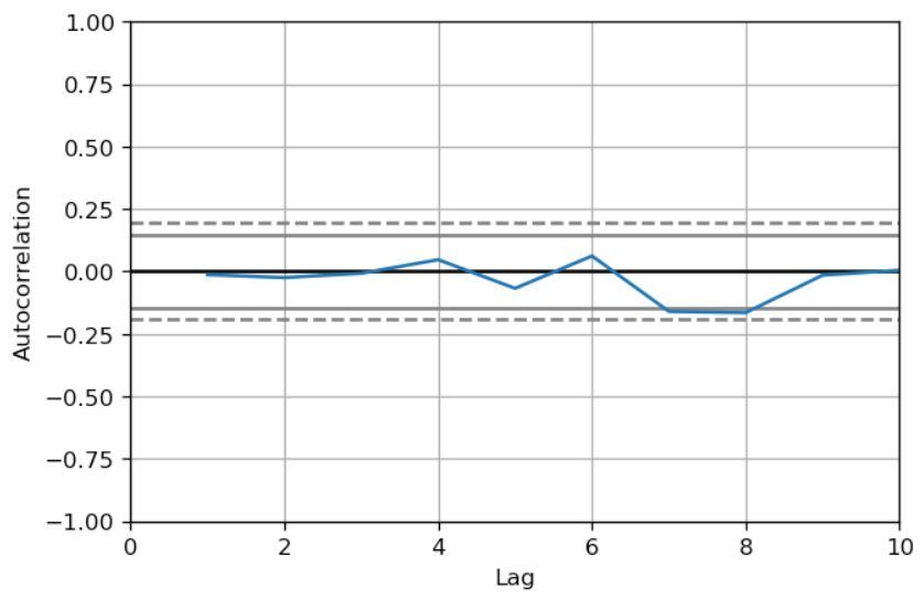
As already discussed the ACF plot is a good way to check autocorrelation in the series.
Looking at the ACF plot it’s possible to detect a high autocorrelation at lag 1. Therefore, this linear model is biased and it’s important to fix this problem.
Cochrane-Orcutt to solve autocorrelation in residuals
The Cochrane-Orcutt procedure is widely used in fMRI data analysis to solve this kind of problem [2]. In this specific case, the lag 1 autocorrelation in the residuals is significant, therefore, we can use the Cochrane–Orcutt formula for the autoregressive term AR(1).
# LAG 0
yt = y[2:180]
# LAG 1
yt1 = y[1:179]

# calculate correlation coef. for lag 1
rho= np.corrcoef(yt,yt1)[0,1]

# Cochrane-Orcutt equation
Y2= yt - rho*yt1
X2 = x[2:180,1:] - rho*x[1:179,1:]
Fitting the transformed Model
Fitting the model again but after the Cochrane-Orcutt correction.
import statsmodels.api as sm

#add constant to predictor variables
X2 = sm.add_constant(X2)

#fit linear regression model
model = sm.OLS(Y2,X2).fit()

#view model summary
print(model.summary())
params = model.params
Now the coefficient X1 is not statistically significant anymore, discarding the hypothesis that the task impact the BOLD signal. The parameters standard error estimate changed significantly, which indicates the high impact of autocorrelation in the residuals to the estimation
Checking for autocorrelation again
This makes sense since it's possible to show that the variance is always biased when there is autocorrelation [1].
Now the autocorrelation of the residuals was removed and the estimate is not biased anymore. If we had ignored the autocorrelation in the residuals, we could consider the coefficient significant. However, after removing the autocorrelation, turns out that the parameter is not significant, avoiding a spurious inference that the task is indeed related to signal.
Conclusions
Autocorrelation in the residuals of a General Linear Model can lead to biased estimates, inefficient predictions, and invalid inferences. The application of the Cochrane–Orcutt procedure to real-world fMRI data demonstrates its effectiveness in removing autocorrelation from residuals and avoiding false conclusions, ensuring the reliability of model parameters and the accuracy of inferences drawn from the analysis.
Remarks
Cochrane-Orcutt is just one method to solve autocorrelation in the residuals. However, there are other to address this problem such as Hildreth-Lu Procedure and First Differences Procedure [1].
Acknowledgement
This project was inspired by Prof. João Ricardo Sato.
The notebook for this article is available here.
References
[1] Applied Regression Modeling, Iain Pardoe. Wileyl. 2023. https://online.stat.psu.edu/stat462/node/189/
[2] Sato JR, Takahashi DY, Cardoso EF, Martin Mda G, Amaro Júnior E, Morettin PA. Intervention models in functional connectivity identification applied to FMRI. Int J Biomed Imaging. 2006;2006:27483. doi:10.1155/IJBI/2006/27483
Solving Autocorrelation Problems in General Linear Model on a Real-World Application was originally published in Towards Data Science on Medium, where people are continuing the conversation by highlighting and responding to this story.
Denial of responsibility! Techno Blender is an automatic aggregator of the all world’s media. In each content, the hyperlink to the primary source is specified. All trademarks belong to their rightful owners, all materials to their authors. If you are the owner of the content and do not want us to publish your materials, please contact us by email – [email protected]. The content will be deleted within 24 hours.